
Introduction
The tracking system has a wide application particularly in the field of navigation where it is useful in manned maneuverable vehicles such as ships, submarines and aircrafts which require accurate tracking. There are various filters employed in these tracking systems. However, in this study focus is on the α - β - γ filter and its optimization in order to improve the prediction of the state variables of the high dynamic target warship.
The theory of the α - β - γ filter has progressed gradually over the years and as its range of applications increase, more and more researchers have expressed quite an interest in the improvement of the design to increase its feasibility and efficiency. Sklasnky(1957) proposed the criteria for determining the performance of a tracking filter as evaluating the stability, noise and computing the maneuvering error. Benedict and Bordner(1962) in their early work established an optimal relationship of the α - β filter’s gain parameters and consequently the filter was known as Benedict- Bordner filter. Later, Simpson et al, (1967) further extended this study by including the acceleration term γ to the α - β filter. Kalata(1984) suggested the tracking index for the α - β - γ filter which defines the optimal set of the smoothing parameters in a closed form. Tenne et al(2002) focused on characterizing the performance of the α - β - γ filter by analyzing the optimal range of the gain parameters. And most recently, ZHENYU et al(2009) uses an improved genetic algorithm (GA) to optimize the initial α , β and γ parameters for application to a non- linear target trajectory. Njonjo et al(2016) employed the α - β - γ filter to track a high dynamic warship and it was proven that the filter was capable of following a highly maneuvering target under a high initial speed with a good degree of accuracy. However, these studies do not specifically define a fixed set of the optimal α , β and γ parameters.
This study proposes the optimization procedure of the α - β - γ filter which involves experimentally plotting the residual error against a set of the damping parameter, ξ. The optimal set of the filtering coefficients is found to depend on the speed of the target in consideration. Simulation results on examination indicate the optimal coefficients corresponding to a particular initial and average velocity.
The α - β - γ tracking filter
The α - β - γ filter is a constant acceleration one stepahead position and velocity predictor that uses the current residual error to predict. The target is assumed to be influenced by zero mean white Gaussian noise. The weighting coefficients α , β and γ are constant therefore reducing the computation time required to maintain a given track.
The α - β - γ filter algorithm involves two major steps of computation as described below Mahafza et al.(2004);.
where
P , V and A are the target’s position, velocity and acceleration respectively.
The subscripts P , S and O denote prediction, smoothing and observation respectively.
n and t denote the sample number and sampling time respectively.
The gain coefficients are determined as follows as extracted from Mahafza et al.(2004);
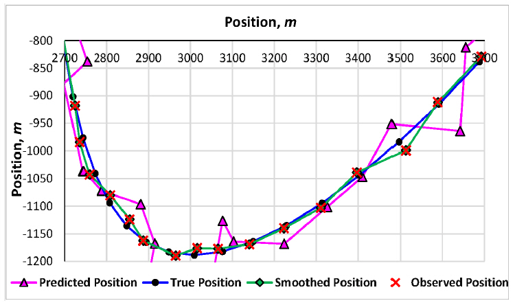
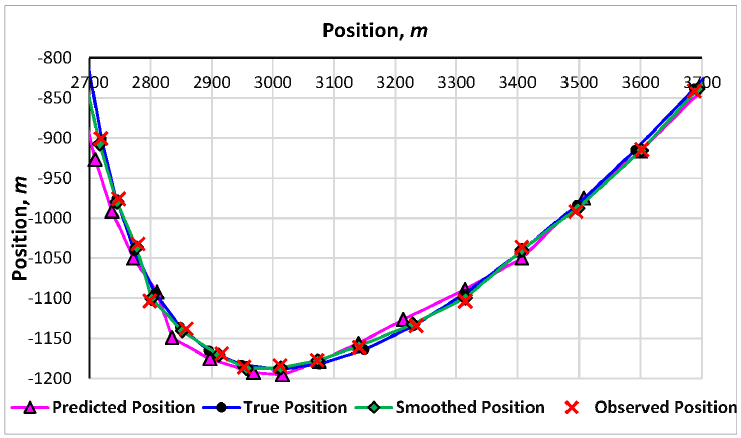
As shown in Eqs. (6) ~ (8), ξ is constrained to lie in the interval [0, 1]. Therefore, when ξ =0, then α=1 and from equation 3, the smoothed position and the observed position are superposed. On the other hand, if ξ =1, then α =0 hence the predicted position and the smoothed position are superposed. This leads to the conclusion that a large ξ results in heavy smoothing. This phenomenon is further illustrated below in Fig. 1, Fig. 2 and Fig. 3. Fig. 1 represents a case of under- damping where the damping parameter, ξ, is very close to zero leading to hardly any smoothing hence the fluctuations on the prediction trajectory throughout the tracking period. Fig. 3, on the other hand, depicts a case of over- damping where the damping parameter is too close to one resulting in lack of sensitivity to target maneuvers. However, Fig. 2, shows a critically damped tracker hence the stability and good sensitivity to target maneuvers.

Simulation
3.1 Target's Initial Conditions
Simulation analysis was carried out on a target whose original observed position lay on the coordinates (573, 1038.4) and was moving at the initial relative speed of 50 m/s as observed from the stationary own ship. The sampling time interval was set at 3 seconds which coincides with the radar scan rate of 20 rpm. A sample size of n=3,000 was investigated. These initial conditions are summarized as shown below in Table 1;
Table 1
Target's initial state
| Position (x, y) | Relative speed m/s | Sampling time intervals, s | Sample size |
|---|---|---|---|
| (573, 1038.4) | 50.4 | 3 | 3,000 |
where a and b are constants that serve to control the initial velocity of the input motion model.
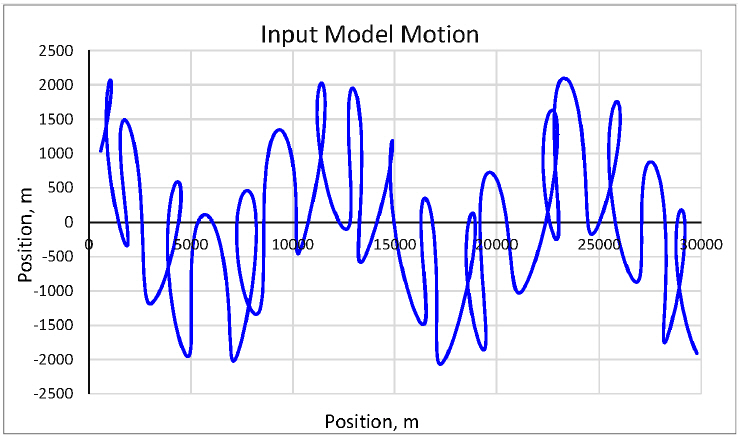
The data was then sampled at intervals of 3 seconds, similar to radar update interval, resulting in the true target’s position trajectory as shown in Fig. 7.
3.2 Noise Addition
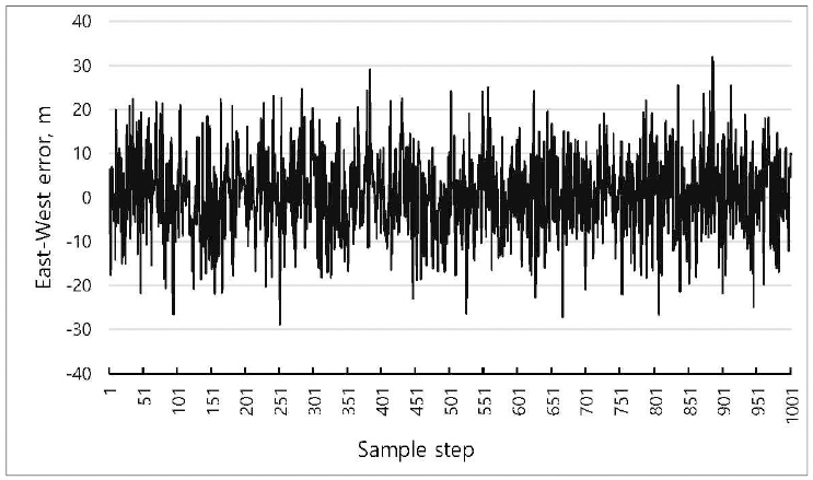
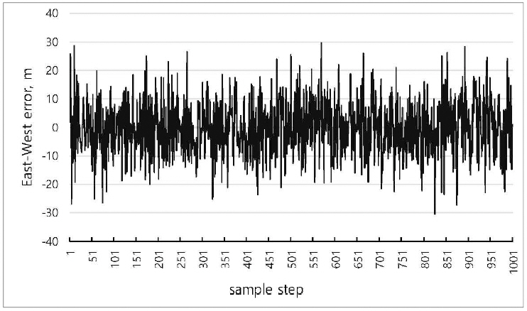
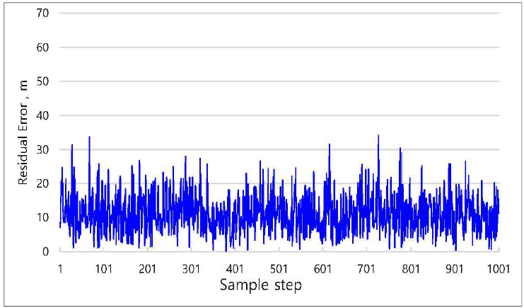
Since the observed position is obtained from the ARPA, the noise cannot be ignore. Generally, the error in the observation follows a normal distribution. In this study, the target’s observed state was obtained by corrupting the true state with zero mean random white Gaussian noise with a standard deviation, σ, of 10 m. Fig. 5 and Fig. 6 show the error distribution in the observation.
3.3 Filter Optimization
The smoothing coefficients α, β and γ values are dependent on the value of the damping parameter, ξ. Therefore, in order to obtain the optimal smoothing coefficients, the ξ is adjusted experimentally until the best value that leads to the best performance is arrived at. Two optimization approaches are investigated in this study, that is, optimization by position and optimization by speed and acceleration.
3.3.1 Optimization by Position.
This method involves comparing the true position, as given in Eq. (9) and Eq. (10), with the predicted position and smoothed position, by calculating the RTP (error between the True and Predicted Position) and RTS (error between the True and Smoothed Position) then plotting the cumulative positional error against a range of the damping factor, ξ. The value of ξ corresponding to the least residual error is the optimal ξ and hence results in the best smoothing coefficients.
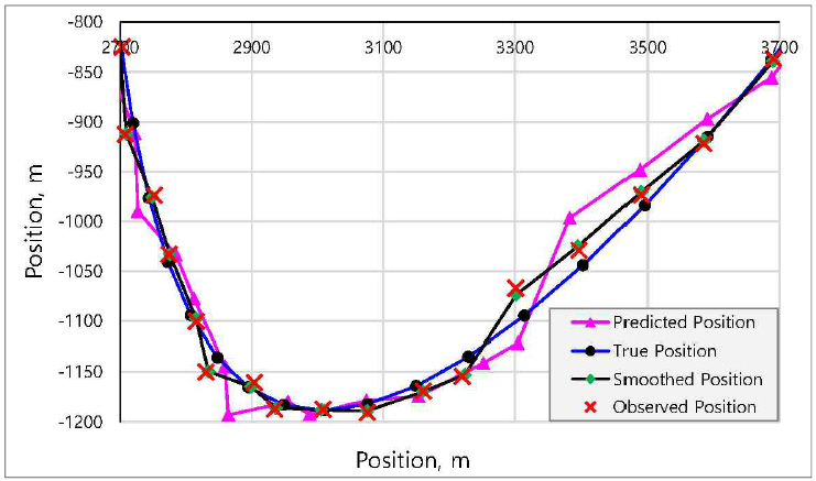
Fig. 7 shows the true, observed, predicted and smoothed positions trajectories. The curve enclosed in the rectangle is enlarged for better viewing as shown in Fig. 8 and lies in the interval [2700, 3700] in the x- axis. Fig. 9 and 10 are the residual errors between the true and predicted and true and smoothed positions respectively corresponding to Fig. 7 and Fig. 8. In this case the damping parameter, ξ was selected arbitrarily as 0.5 for illustration purpose.
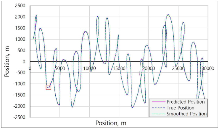
Fig. 8
Enlarged view of target’s true, observed, predicted and smoothed position (ξ =0.5) corresponding to Fig. 7
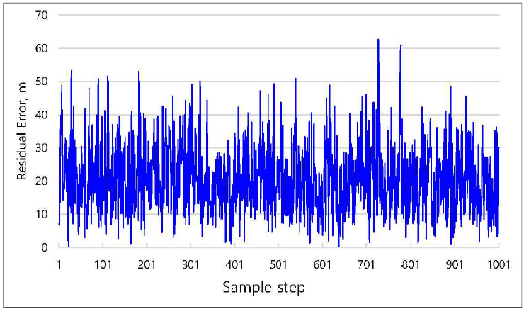
In order to do the evaluation, residual error is used to measure the performance of filter. In this case, residual error indicates the distance between two measurements. For example the residual error T-P indicates the distance between the true position and predicted position. Fig. 9 shows the residual error T-P when ξ=0.5, and the summation of residual error is cumulative error obtained from the whole sample over the given tracking period. To determine the optimal ξ, ξ is set varying from 0 to 0.8 with a step size=0.01. When ξ is beyond 0.8 the residual error increases extremely fast. Fig. 11 shows the summation of residual error T-P while ξ is varying.
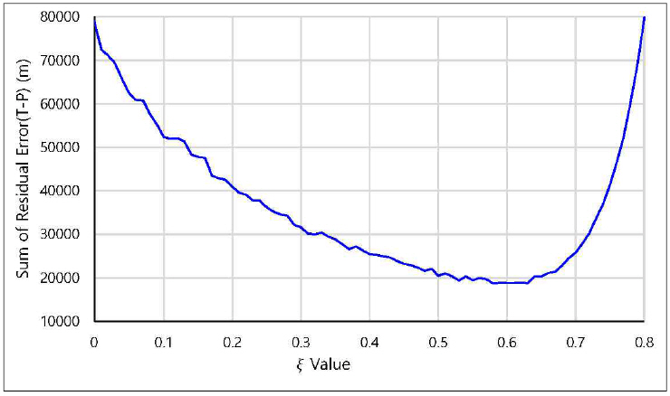
Since random error is used in the above, the curve in Fig. 11 is not smooth. In order to get a relatively smooth curve the simulation is done 30 times. Fig. 12 shows the superposed curves of 30 simulation runs for the summation of residual error T-P. After calculating the average value of summation of each ξ, Fig. 13 can be obtained. It can be clearly seen that when ξ=0.6, the summation of residual error has a minimum point which implies that 0.6 is determined as the optimal ξ by the method of evaluation by summation of residual error of true and predicted position.
Fig. 12
Summation of the error difference between true and predicted positions for varying values of ξ after 30 simulation runs

Fig. 13
Summation of the error difference between true and predicted positions for average values of summation of each ξ corresponding to Fig. 12.
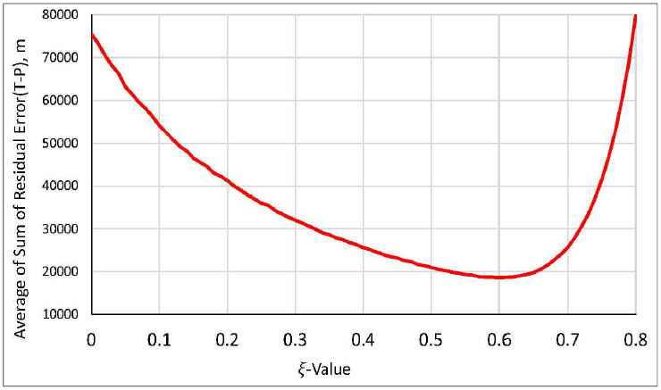
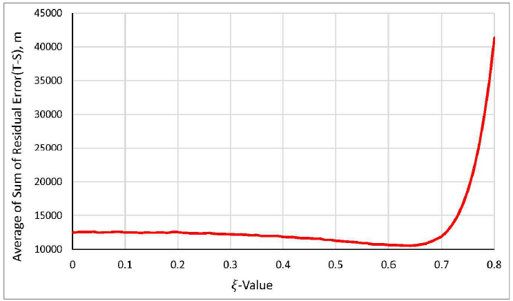
Similarly, when evaluation is done using the summation of residual error T-S (True and Smoothed position), the average value of summation is shown in Fig. 14. The results show that the optimal ξ is 0.64.
3.3.2 Optimization by velocity and acceleration.
The smoothed velocity and acceleration can be obtained after filtering as shown in Eq. (4) and Eq. (5). The first and second derivatives were obtained from Eq. (9) and Eq. (10) resulting in the true target’s velocity and acceleration as shown in Eq. (11) and Eq. (12) respectively. Since the closer the true state variables are to the smoothed variables the better, this method use the residual error of theoretical and smoothed velocity, and the residual error of theoretical and smoothed acceleration to determination the optimal ξ.
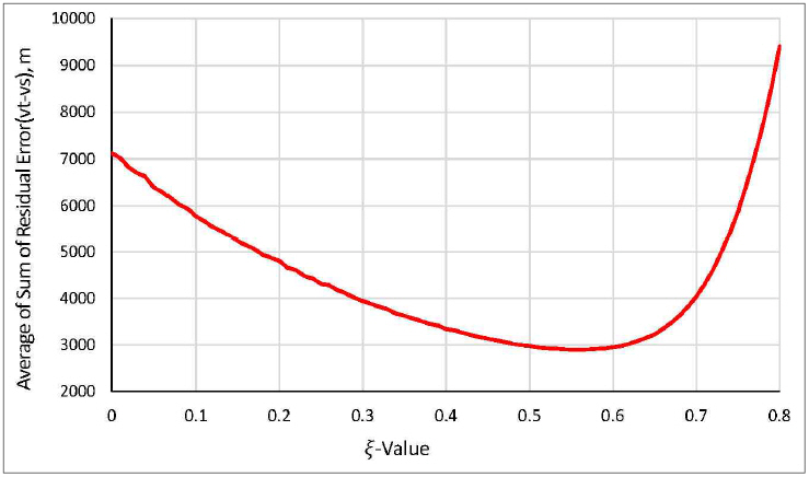
After running 30 simulations and calculating the average summation of residual error of each ξ, Fig. 15 and Fig. 16 were obtained. The minimum point of the curve indicates that optimal ξ is 0.56 on evaluation via residual error of true velocity and smoothed velocity. On the other hand, on evaluation by residual error of true acceleration and smoothed acceleration, the optimal ξ is 0.62 as shown in Fig. 16.

Simulation Results and Analysis
As shown in section 3 above, the initial velocity and the average velocity is a constant value, and the optimized ξ is close to 0.6. From the position Eqs. (9) and Eqs. (10), if the variables a and b change the initial velocity and average velocity will also change.
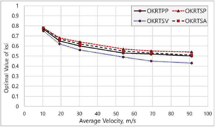
Table 2 below shows the optimal damping parameter obtained for various initial and average target velocities. The quantities a and b serve to control the numerical size of the initial and average target velocity. The results indicate that different relative speeds result in different optimal filtering coefficients. A target model moving at very high initial relative speed requires a low value of the optimal damping parameter compared to a slower target. Fig. 17 is a plot of the optimal damping parameter ξ corresponding to various magnitudes of the average relative velocity.
Table 2
Optimal ξ for varying velocities
Where
OKRTPP: Optimal Evaluated by Summation of the residual error between the true position and predicted position;
OKRTSP: Optimal Evaluated by Summation of the residual error between the true position and smoothed position;
OKRTSV: Optimal Evaluated by Summation of the residual error between the theoretical velocity and smoothed velocity
and,
OKRTSA: Optimal Evaluated by Summation of the residual error between the theoretical acceleration and smoothed acceleration
Conclusion
A high dynamic warship requires accurate tracking and precision in prediction of essential state parameters such as position and velocity. This can only be ensured when an optimal filter is used to carry out the estimation and subsequently the prediction. This study focuses on the optimization of the α - β - γ filter under a noisy environment where the noise is white Gaussian noise with a standard deviation of 10m.
The results indicate that under the conditions of initial target relative speed of 50 m/s, average speed of 30.4 m/s, the optimal ξ for prediction is 0.56 while that of estimation is 0.62. It is further shown that the optimal filtering coefficients are dependent on the initial and the average velocity of the target where different target speeds result in varying smoothing coefficients. In addition, it is clearly indicated that the optimal ξ is inversely proportional to the velocity. Hence, in order to select the best filtering coefficients using the α - β - γ filter, one would have to put into consideration the velocity of the target.
Based on the simulation results, this study proposes that optimal ξ should lie in the interval [0.5, 0.7] when tracking high dynamic warships.
Further analysis of this study will focus on adjusting the optimal ξ at each point of the maneuvering target track to take care of accelerations and maneuvers due to speed changes at specific sample points. This will lead to better filter performance in terms of noise reduction and maintaining a good transient response. In addition the α - β - γ - η filter will be employed to improve the precision of tracking. Finally, the filter will be investigated for tracking the target when both own ship and target warship are in motion.
 PDF Links
 PubReader
 Full text via DOI
 Download Citation
 Print
Print