Basic Study of a Comparison of the Performances of the α-β-γ Filter and the Kalman Filter Regarding Their Use in the ARPA-System Tracking Module of High-Dynamic Warships

Anne Wanjiru Njonjo; Bao-Feng Pan; Tae-Gweon Jeong

doi:10.5394/KINPR.2017.41.5.269

ABSTRACT

“Tracking” here refers to the estimation of a moving object with some degree of accuracy where at least one measurement is given. The measurement, which is the sensor-obtained output, contains systemic errors and errors that are due to the surrounding environment. Tracking filters play the key role of the target-state estimation after the updating of the tracking system; therefore, the type of filter that is used for the conduction of the estimations is crucial in the determining of the reliability of the updated value, and this is especially true since the performances of different filters vary when they are subjected to different environmental and initial conditions. The purpose of this paper is the conduction of a comparison between the performances of the α-β-γ filter and the Kalman filter regarding an ARPA-system tracking module that is used on board high-dynamic warships. The comparison is based on the capability of each filter to reduce noise and maintain a stable response. The residual error is computed from the difference between the true and predicted positions and the true and estimated positions for the given sample. The results indicate that the tracking accuracy of the Kalman filter is higher compared with that of the optimal α-β-γ filter; however, the response of the optimal α-β-γ filter is more stable.

Keywords: α-β-γ Filter, Kalman Filter, Comparison, Performance, Residual Error, Reduce Noise, Stable Response

Introduction

A high dynamic warship is defined by high speed and quick maneuvering. Therefore, accurate estimations of the dynamic parameters are essential for increasing the accuracy of prediction. The Kalman filter is a linear estimator that minimizes the mean squared error as long as target dynamics are modelled accurately. The α - β - γ tracking filter is a third order special case of the Kalman filter that utilizes the tracking error, also known as innovation, to predict the next position. Benedict and Bordner(1962) in their early work established that the performance of the filter relies upon the smoothing parameters α, β and γ.

In the recent past the development of tracking filters has triggered quite an interest from many researchers particularly the performance of the α - β - γ filter and Kalman filter due to their diverse applications in many fields leading to valuable insights into their design improvement. Lawton et al.(1998) distinguished among four types of filtering methods including α - β filter, augmented α - β filter, linear Kalman filter and extended Kalman filter for tracking a non-maneuvering target. Sahoo et al.(2013) compared the performance of α - β - γ filter with Kalman filter for tracking targets using radar measurements and investigated the effects of switching the process noise covariance, Q . Blair et al.(1991) compared the two-stage α - β - γ filter estimator with those of the standard α-β and α - β - γ filters in tracking a maneuvering target whereby the results indicate that the two-stage α - β - γ estimator performs better in the tracking of maneuvering targets hence have increased potential for tracking targets within combat systems that are responsible for tracking and engaging a large number of targets.

This paper aims to compare the performance of both the α - β - γ filter and Kalman filter for tracking a high dynamic target warship from a stationary own ship. The comparison criteria involves comparing the filter’s capability to reduce noise and steadily follow a maneuvering target. In this study, the α - β - γ filter used is an optimal filter designed by (Pan et al., 2016). The Kalman filter employed in this study uses fixed values of the measurement and dynamic noise covariance R and Q respectively.

Methodology

2.1. α - β - γ Tracking Filter Algorithm

The α - β - γ filter is a constant gain, three-state tracking filter. The three-state vector includes position, velocity and acceleration. The acceleration is assumed to be constant and includes zero mean white Gaussian noise.

Mahafza et al.(2004) put forward that the algorithm involves two major stages of computations, that is, prediction and smoothing. Eqs. (1) ~ (3) are the prediction equations for position, velocity and acceleration respectively where they are updated from the estimated state thereby lowering the estimation error. Eqns. (4) ~ (6) are the smoothing equations which are computed by adding a weighted difference between the observed and the predicted position to the forecast state.

Ⅰ. Prediction;

(1)
Pp(n+1)=PS(n)+tVS(n)+t22AS(n),

(2)
Vp(n+1)=VS(n)+tAS(n),

(3)
Ap(n+1)=AS(n).
Ⅱ. Smoothing;

(4)
PS(n)=PP(n)+α(PO(n)−PP(n)),

(5)
VS(n)=VS(n−1)+tAS(n−1)+βt(PO(n)−PP(n)),

(6)
AS(n)=AS(n−1)+2γt2(PO(n)−PP(n)).

where;

the subscripts o, p and s denote the observed, predicted and smoothed state parameters respectively.

P, V and A are the target’s position, velocity and acceleration respectively.

t is the simulation time interval.

n is the sample number.

The selection of the smoothing coefficient is an important design consideration as it directly affects the stability of the output data, error reduction capability and other key design parameters. The α - β - γ filter model under consideration in this study has three real roots and represents the filter minimizing the discounted old data least squares error for a constantly accelerating target whereby the position, velocity and acceleration gain coefficients are determined by the damping parameter, ξ, as shown in Eqs. (7) ~ (9).

(7)

α=1−ξ3,

(8)

β=1.5(1−ξ)2(1+ξ),

(9)

γ=(1−ξ)3.

Where α , β and γ are the position, velocity and acceleration smoothing coefficients, ξ is the damping parameter whose value lies in the interval 0≤ξ≤1. Since the smoothing coefficients are dependent on the value of the damping parameter, optimization of the filter was performed on the ξ by (Pan et al., 2016).

2.2. Kalman Filter Algorithm

The Kalman filter is a recursive filter that requires very little data storage as only the incoming data information is used and therefore does not store up previous information. The Kalman gain is also computed recursively.

The algorithm comprises the following steps;

Ⅰ. Prediction step;

Eq. (10) is the state prediction equation as it predicts the state of the target at time t + 1 based on the state at time t. Eq. (11) is the predicted state covariance matrix of the process noise w_t and it depicts the accuracy of predicting the target’s state at time t + 1 based on the state values obtained at time t.

(10)

Xt+1=FXt+wt,

(11)

Pt+1=FPtFT+Qt,

Where;

X_t = Xt=[xyx˙y˙x¨y¨] is the state vector containing the position, velocity and acceleration parameters and F=[10t0t220010t0t220010t000010t000010000001]

is the state transition matrix.

w_t is the process noise with zero mean and standard deviation σ_w,

Q is the covariance matrix of the dynamic model driving noise vector, w_t

t is the sampling period and

P_t is the state covariance matrix at time t．

The target measurement equation is given by

(12)

Zt=Xt+υt,

Where;

Z_t is the measurement vector which comprises only the position since in this study observation is made on the position only.

υ_t is the measurement error with zero mean and standard deviation σ_υ,

H is the measurement/ observation matrix given by

H=[100000010000].

Ⅱ. Correction step;

Eq. (13) is the Kalman filtering equation as it computes the updated estimate of the current state of the target. Eq. (14) is the updated estimate of the state covariance matrix.

(13)

X^t=Xt+Ktyt,

(14)

P^t=(I−KtH)Pt.

Where;

K_t = PtHSt−1 ; Kalman gain at time t,
y_t = Z_t - HX_t; Residual at time t,
S_t = HP_tH^T + R_t; Residual covariance,
^ denotes the estimated state.

The design of the Kalman filter enables it to easily adapt to changes in noise or sampling intervals while still maintaining optimality since it computes the gains iteratively. This is, however, not the case with the α - β - γ filter whose gains remain fixed at known values. This in turn reduces the computational complexities hence giving the α - β - γ filter an advantage over the Kalman filter.

Simulation

3.1. Target model conditions

The target was modeled under the initial conditions laid out in Table 1 below.

Table 1

Target’s initial conditions

Position (x, y)	Relative speed m/s	Sampling time intervals, s	Sample size
(573,1038.4)	50.4	3	1,000

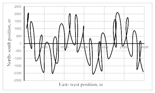
The original high dynamic target’s position was modeled using the sine-Cosine equations shown below in Eqs. (15) & (16);

(15)

Xi=a[10 sin(1.2wi)]+7cos(0.99wi)+8sin(0.7wi)+6 cos(2wi)+9 sin(3wi)+5 cos(3wi)+10i,

(16)

Yi=b[20 cos(0.3wi)+22 sin(2wi)].

Where parameters a and b in the above are applied to control the relative speed in this study.

The resulting data was then sampled at intervals of 3 seconds to give the true trajectory of the target as shown below in Fig. 1.

Fig. 1

Target’s true position

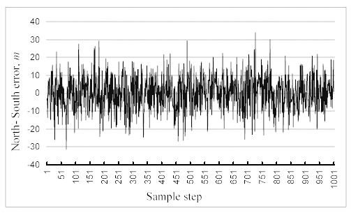
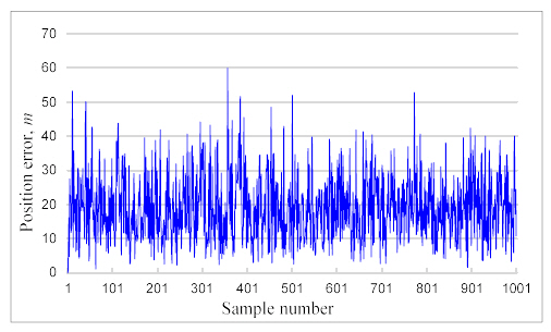
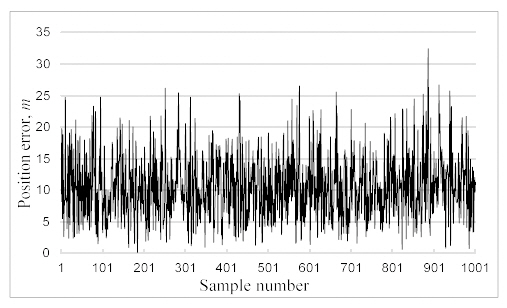
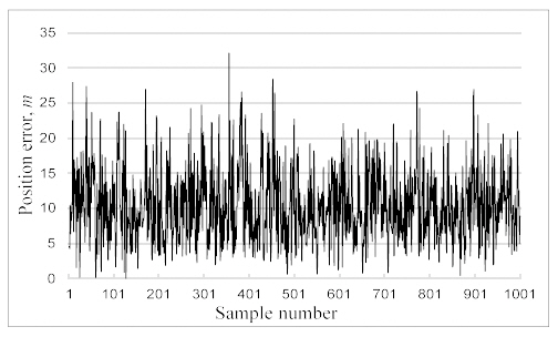
3.2. Noise Addition

The observed position is the output obtained from the radar measurements and therefore includes an error. In this study, the noisy observation was obtained by corrupting the true state with zero mean random white Gaussian noise with a standard deviation, σ, of 10 m. Fig. 2 and Fig. 3 show the error distribution in the observation.

Fig. 2

East-West error in the observation

Fig. 3

North-South error in the observation

3.3. The α, β and γ Selection

The filtering coefficients, α , β and γ, were chosen based on the optimal value of the damping parameter ξ. Pan et al.(2016) suggested that the damping parameter ξ should be set as 0.64 for a maneuvering target with an initial speed of 50.4 m/s . Equations (5) ~ (7) were then employed to compute the optimal filtering coefficients. Therefore, the α - β - γ filter used in this study for comparison is an optimal filter.

3.4. Kalman Filter Tuning

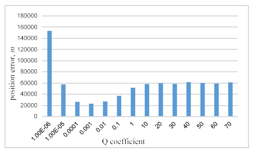
The R matrix shows the accuracy of the radar measurement. Hence, it is the covariance matrix of the measurement error, υ, with a variance of υw2. The matrix Q , on the other hand, reflects the uncertainty in the target’s trajectory and therefore it is the process noise, W, covariance matrix with a variance of σw2. Since the effects of both R and Q are negatively correlated, the matrices need to be carefully selected and tuned to avoid divergence of the filter estimates rendering them useless. In addition, given that the R and Q matrix in this study are a fixed value throughout the filtering process, the initial choice of both covariance matrices is crucial in ensuring a good performance of the filter.

The tuning process in this study was achieved by changing the Q and R covariance matrices while simultaneously feeding the measurement data to the filter for each covariance matrix coefficient. The output was then used to compute cumulative positional error which was then plotted against corresponding covariance matrix coefficients. The purpose of this was to identify the covariance matrix coefficient corresponding to the least error. From the Fig. 4 and Fig. 5, the values of R and Q covariance matrix coefficients corresponding to the minimum residual error are 1 and 10^-3 respectively.

Fig. 4

Cumulative error difference between observed and predicted positions against R matrix coefficient

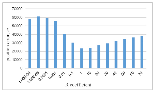
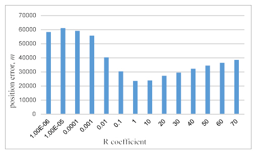
Fig. 5

Cumulative error difference between true and smoothed positions against R matrix coefficient

Fig. 6

Cumulative error difference between observed and predicted positions against Q matrix coefficient

Fig. 7

Cumulative error difference between true and smoothed positions against Q matrix coefficient

Comparision of the filters

In this study, comparison of the two filters’ performance was made based on the filter’s capability to minimize the noise level and ability to follow the randomly maneuvering target warship. This was done by comparing the size of the error in the estimated and predicted positions, that is estimation and prediction error respectively. Estimation error is obtained by computing the deviation of the estimation from the true position for each sample. Similarly, prediction error indicates how far the predicted position deviates from the true position.

Fig. 8 & Fig. 9 show the true, observed, predicted and smoothed positions trajectories. Fig. 8 shows the positional trajectories obtained from the α - β - γ filter, while Fig. 9 shows the resulting trajectories for the Kalman filter. From the curves, the α - β - γ filter seems to easily follow the maneuvering target warship with greater sensitivity as indicated by the steadiness in the predicted and smoothed trajectories. On the contrary, the predicted and smoothed curves resulting from the Kalman filter are marred with erratic changes and overshooting at various points on the trajectories indicating the filter’s inability to respond well to maneuvers particularly for this type of trajectory.

Fig. 8

Target’s True, Observed, Predicted and Smoothed Position (ξ=0.64), α - β - γ filter

Fig. 9

Target’s True, Observed, Predicted and Smoothed Position, Kalman Filter

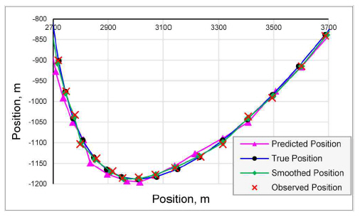
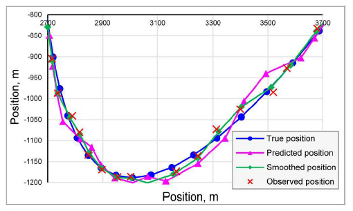
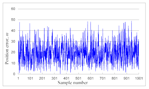
Fig. 10 & Fig. 11 show the cumulative prediction errors resulting from the α - β - γ filter and the Kalman filter respectively. Fig. 12 & Fig. 13 are the cumulative estimation errors obtained from the α - β - γ filter and the Kalman filter respectively. These results show that the Kalman filter has a slightly higher accuracy in both prediction and estimation of the position of the target warship than the α - β - γ filter.

Fig. 10

Cumulative prediction error, α - β - γ filter, error= 19, 622 m

Fig. 11

Cumulative prediction error, Kalman filter, error=19,104 m

Fig. 12

Cumulative estimation error, α - β - γ filter, error=10,653 m

Fig. 13

Cumulative estimation error, Kalman filter, error=10,492 m

Conclusion

In this study, two filters have been considered for comparison in their performance. The results obtained depict that both filters when properly designed and tuned are capable of tracking the high dynamic warship with some degree of accuracy. The Kalman filter, however, has a higher accuracy in both prediction and estimation of the target’s position as compared to the optimal α - β - γ filter. On the other hand, the smoothed and predicted trajectories obtained from the Kalman filter appear to have a high rate of overshooting from one sample point to another along the trajectory hence unstable. The α - β - γ filter smoothed and predicted trajectories are steady throughout the whole sample indicating its ability to respond well to the target’s maneuvers. In addition, the optimal α - β - γ filter given its ease of implementation due to a low computational load performs quite competitively when compared with the Kalman filter.

Future study will involve tracking the high dynamic target warship while own ship is also on motion. In addition, the authors will consider replacing the α - β - γ filter with the four-state filter α - β - γ - η filter for a more precise prediction.