1. Introduction
The IMO has already mandated the onboard carriage of the automatic identification system (AIS) since 2004. With this equipment, the AIS information of ship in a navigating area can be exchanged with other ships to ensure maritime safety. Moreover, the ships are also required to frequently transmit AIS messages to the VTS station. This information can be used for purposes such as the avoidance of ship collision in the harbour and assist with traffic operation in the fairway, to gain the statistics about the density traffic, to support maritime accident investigation and so on. In some situations such as when navigating in a busy coastal area, faults with transmitter are to be expected because of difficulties occurring when, the capacity of VTS station is overloaded in a crowded area, the VTS station can't handle dealing with AIS information from all the ships as standards, therefore it is necessary to have interpolation methods for recovering missing AIS information.
In recent years, some research has been carried out on interpolating and predicting the ship's state, however, when applying these to recover missing AIS data, some problems still remain. Firstly the given results in which a large errors occur, the interpolated parameters such as COG, SOG and HDG haven't yet been set out as sufficiently and accurately as they would be through an AIS message secondly each method is only suitable for some types of AIS data, and finally in areas of strong wind and currents, the parameters of the AIS dynamic change very quickly, so modelling the variation of a ship’s dynamic based on its physical characteristics is very difficult. In (
Perera, 2010) the theory of the Kalman filter was applied to predict the optimal parameters of the velocity and the acceleration of the ship, but this approach just described the maneuvering situation of the ship in ocean which is not suitable for interpolating the missing AIS data. The Neural network was employed to predict the ship’s trajectory (
Xu, 2012) however, the structure of neural networks is uncertain in its capacity to model the characteristics of ship movement, moreover, the results of this haven’t yet been shown clearly in this research. Therefore in using the neural network it is hard to meet the demand to interpolate the missing AIS data problem. The vector motion function and parametric curve model for interpolating the ship's state was proposed by (
Hu, 2014) in which the odd order-polynomial functions and derivatives are used to build the model, however, in this method, the heading line was always has to be fixed to the tangents of the ship’s trajectory, however this is in fact not always true, this method just considers three parameters including the ship position, ship's heading and the ship's speed.
This research proposes a method which includes linear interpolation, cubic Hermit interpolation and an identification mechanism for interpolating the missing AIS data of a ship. The proposed method can be suitable for many different kinds of lost data, as long as the parameters are interpolated sufficiently as an AIS message. Firstly, all the given AIS data such as ship position, COG, SOG and HDG is divided into separate time series, and then the characteristics of the missing data is investigated by an identification mechanism, and finally the appropriate interpolation which fits all the time series is selected. Numerical experiments are carried out using real AIS data to validate the algorithm of this approach and to compare the results with the previous methods. After which, the actual missing area to be interpolated is indicated by the proposed method. The interpolation results show this approach can be applied well in practice.
2. The requirement of transmitting AIS data for autonomous mode
The AIS data is divided into three areas: static data, dynamic data and related information as expressed in accordance with the international standard (
IEC61993-2, 2001). The first one includes the following: the ship name, MMSI number, ship’s IMO number, call sign, the length and beam, type of vessel, route plan, AIS type, the second one consists of the ship position, UTC time, course over ground (COG), speed over ground (SOG), heading angle (HDG), rate of turning (ROT), the heeling angles. Finally, some information related to the voyage with regard to the vessel’s draft, port of destination and estimated time of arrival and the route of transition also exchanged in AIS system, detailed illustration in Fig.
1.
Fig. 1
The static and dynamic of AIS message
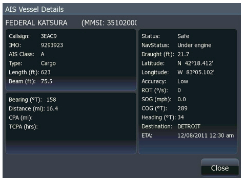
In this research, the dynamic information such as the ship position, COG, SOG and HDG are considered for interpolating the problem of missing AIS data. As the regulation stipulates, in autonomous mode, the static information should be transmitted every 6 minutes when data has been amended and on request, the dynamic information depends on the ship’s speed and course alteration, the requirement of transmitting AIS dynamic data is expressed in the international standard (
IEC61993-2, 2001) as below Table
1.
Table 1
Information update rates for autonomous mode
|
Type of Ship |
Reporting Interval |
|
Ship at anchor or moored and not moving faster than 3 knots |
3 mins |
|
Ship at anchor or moored and moving faster than 3 knots |
10 seconds |
|
ship with a speed of between 0 - 14knots |
10 seconds |
|
ship with a speed of between 0 - 14knots and changing course |
3 1/3 seconds |
|
ship with a speed of between 14 -23 knots |
6 seconds |
|
ship with a speed of between 14 - 23 knots and changing course |
2 seconds |
|
ship with a speed of greater than 23 knots |
2 seconds |
|
ship with a speed of greater than 23 knots and changing course |
2 seconds |
3. Numerical method for interpolation missing AIS data of ship
The interpolation method is proposed to recover missing AIS data based on the AIS data which was received before and after the missing time interval, it can be seen in Fig.
2.
Fig. 2
The missing AIS dynamic data of ship
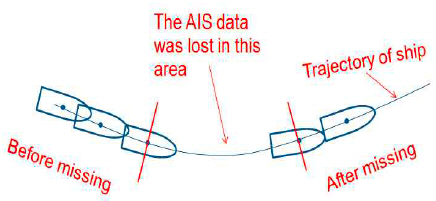
Firstly, all of the ship’s dynamic parameters in the AIS message are divided into the five following separate time series (ti, lat(ti)), (ti, long(ti)), (ti, COG(ti)), (ti, SOG(ti)), (ti, HDG(t1)). To simplify the algorithm analysis regarding the missing AIS, the (ti, fi ) symbol is used to represent all time series used in the construction of the interpolation method. In this section, the mathematical theory of interpolation as well as the identification of the characteristics of the AIS time series are considered. Let’s say Ai (ti, fi) is the data resulting from the AIS time series. When the shape of the time series is nearing a straight line, the linear interpolation is used, in the case of curve shape or in the case of the parameters of the ship's dynamic changing quickly, the curved interpolation should be applied.
3.1. Piecewise Linear Interpolation
Piecewise linear interpolation is adopted in recovering the missing points of the AIS time series. Every two adjacent points
Ai (
ti,
fi ) and
Ai+1 (
ti+1,
fi+1 ) in time series give one piece, the piece of one track can be drawn as a straight line (
Lin, 2007). The general formula of piecewise linear interpolation is presented as Eq.(
1).
Where
Pi (
t) is one piece between two points of a time series
Ai (
ti,
fi ) and
Ai+1 (
ti+1,
fi+1) , the time
t is within [
ti,
ti+1]. The function
Pi (
t) can be determined as Eq.(
2).
3.2. Piecewise Cubic Hermite Interpolating
In order to preserve the shape of the data, this interpolation method is proposed, it is good for interpolating the time series which has characteristics of the curved shape. In this research, the cubic Hermite interpolation polynomial is used for this purpose. The cubic Hermite interpolation is formulated as (
Lin, 2007). Let
s,
h are respectively the local variable and the length of the
ith subinterval, they are defined as Eq.(
3).
The
di,
di+1 symbols denote the slope of the interpolant at
ti,
ti+1 , they satisfy Eq.(
4) and Eq.(
5) as follows
The cubic Hermit polynomial on interval
ti ≤
t ≤
ti+1 can be represented as below Eq.(
6).
This is a cubic polynomial in
s, and hence in
t, that satisfies four interpolation conditions, two on function values and two on the possibly unknown derivative values, they are represented as Eq.(
7).
3.3. Identification of the characteristic of AIS time series
According to the current ship's speed and the transmitting time of the AIS signal, we can find out the missing area of AIS data and how many points were lost. However, to recognize whether the ship is on a steady course or turning course, the curvature of the time series is investigated in following section. In (
Karl, 2009), the formula of curvature is generally constructed as Eq.(
8).
In Cartesian coordinate system, the formula for curvature is presented as Eq.(
9).
Eliminating the
dϕ/
dt, using the angle between two tangents as Eq.(
10).
Substituting Eq.(
11), Eq.(
10) into Eq.(
9), the final curvature calculated from the x and y in Cartesian coordinate system, represented by the Eq.(
12).
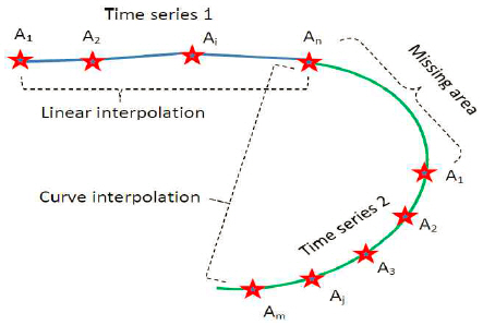
The AIS time series can be identified by its straight or curved shape. Firstly, the mean curvature values of both the time series before and after the missing area are calculated as
κ1,
κ2, anymore the standard deviation of them is also determined as
σ1,
σ2. Secondly, if
κ2 is outside the band
κ1 ± 2
σ1, it means that the AIS time series changes her course due to missing the area so a kind of curve interpolation is applied, and in the other cases the linear interpolation should be used. The illustration is shown as Fig.
3.
Fig. 3
Identification of characteristic of AIS time series
3.4 Algorithm of interpolation method for missing AIS data
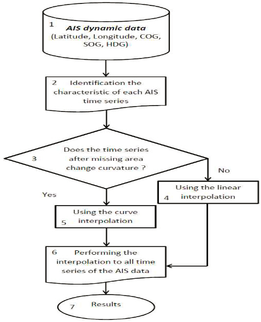
The above Fig.
4 shows the block diagram of the interpolation method for missing AIS data, the function of blocks are explained as follows. In the block of AIS dynamic data, all parameters of the AIS data are divided separately into time series which include latitude, longitude, COG, SOG and HDG. After that, the block identification of the characteristics of each AIS time series will calculate the curvature of time series before and after the missing area and check the time series whether time series is straight or curved shape. Next step is the decision of whether to use linear or curve interpolation and it is carried out in the block of checking the curvature change. Then, the block of linear and curve interpolation provides a concrete method for the missing area. Finally, all time series of AIS data are interpolated and combined in a block of performing the interpolation to all the time series of the AIS data.
Fig. 4
The block diagram of the interpolation method
4. Numerical experiment and results comparison
In this part, the numerical experiment is carried out to verify the performance of the proposed method. The real time data is collected from the Sewol passenger ferry of South Korea, which sunk at JinDo island in April-16, 2014. The real time AIS data at the certain time interval is chosen to validate the reliability of the proposed algorithm. In addition, the method of the vector motion function is also employed to compare the results with the proposed method.
After that, the actual area where the ship lost her AIS data is indicated by interpolating this method and the validation area and the suggestions resulting from AIS data is illustrated in Fig.
5.
Fig. 5
The trajectory of Sewol passenger ferry
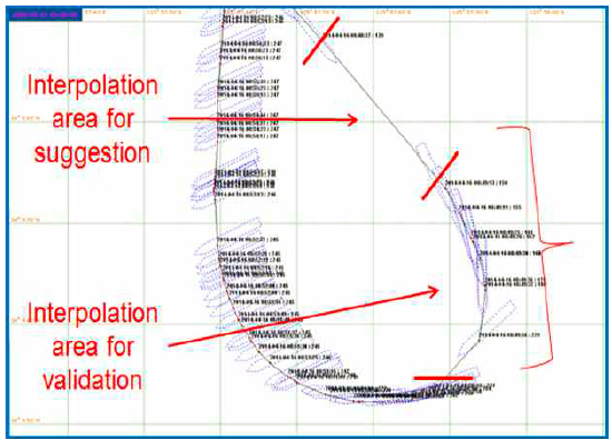
4.1. Interpolation of missing AIS data for validation area
To verify the accuracy and the feasibility of this method, some experiments are adopted for the validation area. Table
2 shows the real time-9 points of AIS data, from 08:48:44 AM to 08:50:10 AM which was assumed to be the missing area of AIS data. Then the interpolation method (
John, 2004) is applied to validate its performance in this area. All of the time series such as latitude, longitude, COG, SOG and HDG in this experiment consisted of 200 time samples taken out from between 08:46:52 AM to 09:19:23 AM in which, the first sample, the time is assumed as (t = 0). However, for easier viewing, only the first 90 time samples are shown, from 08:46:52 AM to 08:58:13 AM which contains both the validation and the suggestion area. Moreover, the figures of the time series are plotted to clearly illustrate the area of the missing AIS data.
Table 2
The real time-9 points for interpolation at the validation area
|
Time |
Ship position Latitude (N) Longitude (E) |
COG (deg) |
SOG (knots) |
HDG (deg) |
|
08:48:44 |
34°9'51.7" 125°57'45.6" |
134 |
17.3 |
140 |
|
08:49:13 |
34°9'44.08" 125°57'53.7" |
146 |
17.1 |
150 |
|
08:49:40 |
34°9'37.50" 125°57'56.7" |
175 |
15.5 |
184 |
|
08:49:44 |
34°9'36.9" 125°57'56.6" |
182 |
15.1 |
199 |
|
08:49:45 |
34°9'36.65" 125°57'56.5" |
183 |
15 |
213 |
|
08:49:47 |
34°9'36.48" 125°57'56.7" |
182 |
15 |
191 |
|
08:50:00 |
34°9'34.38" 125°57'55.9" |
206 |
13.4 |
234 |
|
08:50:06 |
34°9'33.30" 125°57'54.9" |
224 |
11.8 |
242 |
|
08:50:10 |
34°9'32.93" 125°57'54.5" |
228 |
11.5 |
246 |
Besides these 9 points, there are some others. The time interval between first point and second point is the actual missing area (29 seconds). Between second point and third point, 6 other points also belonged to this time interval (27 seconds). The time series before and after the missing area of AIS data is shown in Fig.
6, Fig.
7, Fig.
8, Fig.
9 and Fig.
10. The time series of latitude and longitude in Fig.
6 show the blank area, by viewing and calculating the curvature of these time series. These are before and after missing area and the linear interpolation is used to fit the data for the time series of latitude and longitude in two first points, the curve interpolation is used for remaining points. The result is presented in Fig.
7, where the dot symbol denotes given data, the circle one is the interpolated result.
Fig. 6
Latitude and longitude data before interpolation
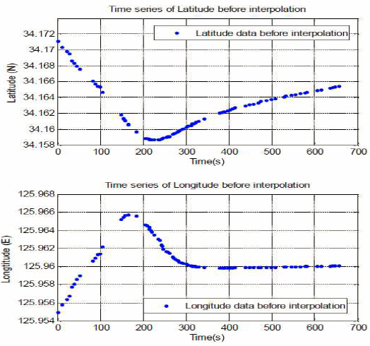
Fig. 7
Latitude and longitude data after interpolation
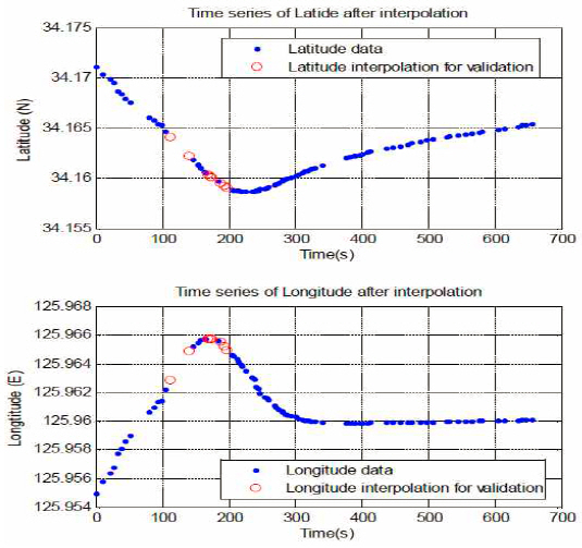
Fig. 8
The COG, SOG, and HDG data before interpolation
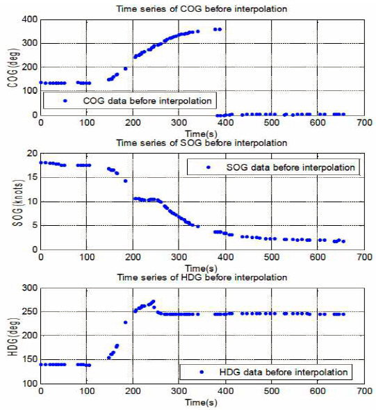
Fig. 9
The COG, SOG and HDG data after interpolation
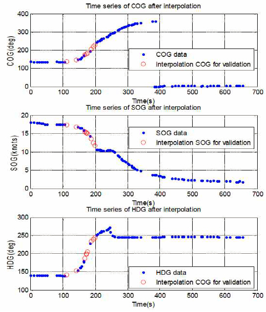
Fig. 10
The ship's trajectory after interpolating for validation area
Similarly, the time series of COG, SOG and HDG before the missing area are shown in Fig.
8. The curve interpolation is applied for these time series.
The results of interpolation for these blank areas are presented in Fig.
9, the dot symbol is given data, the circle symbol denotes interpolated result.
The detailed results of the validation area interpolated by this method are shown in Table
3.
Table 3
The results of interpolation for validation area
|
Ship position Latitude (N) Longitude (E) |
COG (deg) |
SOG (knots) |
HDG (deg) |
|
34°9'50.4" 125°57'47.48" |
135.1 |
17.5 |
139 |
|
34°9'43.92" 125°57'53.89" |
146.6 |
17.0 |
150 |
|
34°9'37.44" 125°57'56.80" |
176.1 |
15.3 |
186.8 |
|
34°9'36.72" 125°57'56.88" |
181 |
15.0 |
197.4 |
|
34°9'36.36" 125°57'56.88" |
182 |
14.9 |
200.2 |
|
34°9'36.36" 125°57'56.84" |
184 |
14.8 |
205.9 |
|
34°9'34.20" 125°57'55.72" |
203.2 |
13.6 |
235.8 |
|
34°9'33.48" 125°57'54.65" |
218.4 |
12.2 |
242.7 |
|
34°9'32.76" 125°57'53.86" |
229 |
11.3 |
246 |
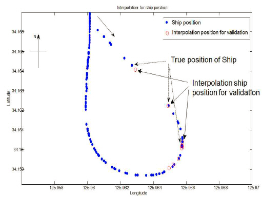
The trajectory of the ship after interpolating in the validation area is shown in Fig.
10 and Fig.
11, where the dot is true position of ship and the circle is interpolated position.
Fig. 11
The interpolated ship position for validation area
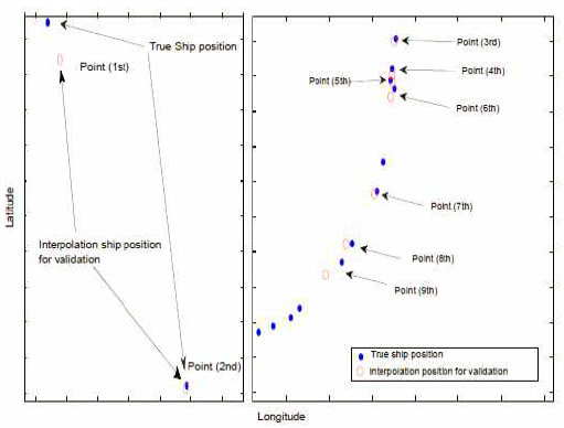
The left of Fig.
11 shows the two first points of ship position which are interpolated by the linear method, and the other one presents 7 points of a ship position to be interpolated by curve interpolation.
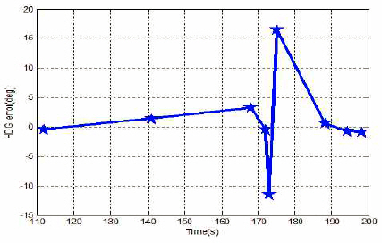
The absolute error is determined at 9 points by comparing interpolated results with actual data of the AIS time series in order to show the error of the proposed method, and then average error is also calculated for these 9 points. Then results of the errors are presented as Fig.
12, Fig.
13, Fig.
14 and Fig.
15.
Fig. 12
The error of ship position interpolation
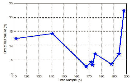
Fig. 13
The error of COG interpolation
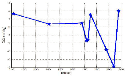
Fig. 14
The error of SOG interpolation
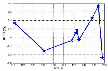
Fig. 15
The error of HDG interpolation
After completing the interpolation for the validation area by the proposed method, the vector function method is also employed with this data and the results given by two methods are compared to each other, shown as Table
4.
Table 4
The average error of two interpolation methods
|
Method |
Average position error |
Average COG error |
Average SOG error |
Average HDG error |
|
The purposed method |
7.23(m) |
1.89 (degree) |
0.15 (knots) |
3.95 (degree) |
|
Vector function method |
15.7(m) |
X |
0.6 (knots) |
8.14 (degree) |
From the results, we can consider the following outcomes. Firstly, it is not possible to obtain the value of the course over ground (COG) in the vector function method Secondly, while the proposed method in this paper applies the adaptive mechanism which can choose the appropriate interpolation method, the vector function method uses only the curve model. Therefore the error of ship position, SOG and HDG given by the proposed method is found to be smaller than those given by the vector function method. Thirdly, the HDG of the vector function method is not always same as the true heading angle because the heading line is used in a way which is always at a tangent to the ship's trajectory in the vector function method.
4.2. Suggestion of interpolation method for actual missing area of AIS data
From 08:48:44 AM to 08:49:13 AM, the AIS data of ship is completely lost. In this part, the interpolation method is suggested for recovering the missing data of this area. Ship positions in this part are shown in Fig.
16, the result of this area is presented in Table
5.
Fig. 16
The trajectory of ship in suggestion area
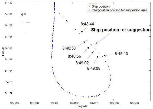
Table 5
The results of interpolation for suggestion area
|
Time |
Ship position Latitude (N) Longitude (E) |
COG |
SOG |
HDG |
|
08:48:50 |
34°9'49.12" 125°57'48.24" |
137 |
17.4 |
141 |
|
08:48:56 |
34°9'47.72" 125°57'49.86" |
139 |
17.3 |
143 |
|
08:49:02 |
34°9'46.41" 125°57'51.3" |
141 |
17.1 |
146 |
|
08:49:08 |
34°9'45.12" 125°57'52.63" |
144 |
17 |
148 |
Based on the ship's speed and the characteristics of the time series, the linear interpolation is applied for interpolating 4 points of the ship position and the curve interpolation for COG, SOG and HDG of AIS data in this area.
5. Conclusion
The conclusion of this research can be summarized as follows
- This research proposes one method for interpolating the missing AIS data of ships based on numerical interpolation and the characteristics of the AIS time series.
- All parameters such as the ship position, course over ground, speed over ground and the heading angle are interpolated sufficiently by this method.
- This method includes linear interpolation, cubic Hermit interpolation and an identification mechanism, so it has an adaptive ability to many shape AIS data.
- Experiments show that the results of this method are better than in the previous method in interpolating the AIS data problem.
- In the future, the dynamic characteristics of the ship according to the kinematic equation and the disturbance of current and wind will also be considered to improve the ability to predict the missing area which has wide time range.


 PDF Links
 PubReader
 Full text via DOI
 Download Citation
 Print
Print