Lead-lag Relationship between the Shipping Freight Rate and Agricultural Commodity Import Price in Korea

Article information

J Navig Port Res. 2021;45(2):69-74

Publication date (electronic) : 2021 April 30

doi : https://doi.org/10.5394/KINPR.2021.45.2.069

Jae-Young Ha ^*^,, Youngran Shin ^†^,

^*Expert, CJ Foodville, Busan, South Korea

^†Associate Professor, Graduate School of Global Logistics, Korea Maritime and Ocean University, Busan, South Korea

^†Corresponding author, syran@kmou.ac.kr 051)410-4486

^*hjy987@hanmail.net 051)990-7982

Received 2021 February 21; Revised 2021 March 9; Accepted 2021 March 10.

Abstract

This study aims to investigate the lead-lag relationship between the agricultural produce import price in Korea and the corresponding shipping freight rate. Since the Korean economy has pursued an export-driven growth strategy, mainly based on the manufacturing sector, the country has to depend on the vast majority of its agricultural produce consumption after import from foreign countries. Moreover, compared with other high-value products, transportation cost occupies a substantial share of the agricultural commodity price, resulting in changes in the shipping freight rate being a pivotal determinant of agricultural produce import. In this respect, this study explores the possible association between agricultural produce import in Korea and shipping freight rate and the lead-lag relationship. Using a monthly dataset of agricultural produce import prices and freight rates for Handysize and Panamax dry-bulkers for the period between J anuary 2010 and November 2020, this study determines that the shipping freight rate, in general, leads the agricultural commodity price.

Keywords: commodity price; freight rate; granger causality; lead-lag relationship; vector autoregression

1. Introduction

This study aims to examine the lead-lag relationship between the agricultural produce import price of Korea and corresponding the shipping freight rate, exploring the impact of logistics costs on the price of cargo transported. The success of the export-driven growth strategy has contributed to the remarkable economic development of Korea for the past several decades. Nowadays, Korea ranks as a global top-tier economic power in terms of GDP, GDP per capita and international trade.

However, at the same time, since the economic policy of Korea stresses out the importance of the manufacturing sector, the competitiveness of other sectors relatively has diminished. This phenomenon is especially evident in the primary industries, such as, mining, agriculture and forestry. Therefore, Korea has to depend its food consumption on import from other countries, resulting in the food self-sufficiency rate being below 50% (see Fig. 1). The supply of food becomes more serious considering the fact that the degree of grain self-sufficiency (the concept includes nutrient for human-being food consumption and animal feed) is 21% in 2019. Consequently, the Korean economy is vulnerable to volatility in the international agricultural produce prices and access to food resources is a critical factor even for national security in times of emergency.

Fig. 1.

Food and Grain Self-Sufficiency Rates of Korea Source: Korea Rural Economics Institute

Therefore, the investigation of factors affecting the prices of agricultural commodities imported into Korea is of utmost importance. In this regard, this study pays particular attention to the association between the shipping freight rate and the import price of agricultural produce of Korea and the possible causal relationship between the two factors. It is quite self-evident that there exists a close relationship between the agricultural price and the freight rate as the vast majority of the country’s export and import is serviced by shipping transportation. Although a voluminous body of research has been done in this subject, there has been, to the best knowledge of authors, no attempt to investigate the lead-lag relationship in the case of Korea. By examining the under-explored area, the findings in this study can offer important implications for both academic and business alike.

The rest of this paper is structured as following: Section 2 reviews previous literature. Section 3 explains methodology and data used in analysis. Section 4 presents the empirical evidence. Finally, Section 5 concludes.

2. Literature review

The role of shipping freight rate as a leading indicator has long been a thought-provoking agenda in the economic study. In this regard, a strand of research pays academic attention to freight rates in the dry bulk and oil tanker sectors since these two types of ships serve transportation of raw materials, such as iron ore, coal, grains and crude oil, to name a few. The rationale is that the consumption of those commodities can stimulate industrial production, so that, the changes in shipping freight responding to fluctuations in demand for raw materials can signal economic situation in the near future.

Bakshi et al.(2011) find that Baltic Dry Index (BDI) can be used as a leading indicator for the global stock index, the commodity price and the economic cycle. Similarly, Bildirici et al.(2016) investigate the predicting power of BDI for the period of January 1985-March 2015. It is found that there is long-run equilibrium among BDI, gold price and the GDP of the USA. In the case of Korea, Lee and Kim(2014) report a bi-directional causality between BDI and KOSPI, the major stock market index of Korea, during 2006-2013. Kim et al.(2016) find a negative association between shipping freight index (BDI, China Containerized Freight Index, Howe Robinson Containership Index) and the stock price of Korean shipping companies, which arguably indicates the inappropriate response to shipping market cycles. Furthermore, Kim and Shin(2018) document that freight rate indices for the dry bulk sector, such as BDI, Baltic Capesize Index and Baltic Panamax Index (BPI), have a significant predictive power for the volume of international trade of Korea. In addition, Kim and Oh(2012) find the existence of long-run relationship between BDI and stock prices of Korea shipping companies.

Another strand of research highlights the lead-lag or the causal relationship between the shipping freight rate and the prices of commodities transported. Kavussanos et al.(2014) explore the lead-lag relationship between derivatives prices of shipping freight and agricultural commodities and find that commodity price informationally leads shipping freight rate. Moreover, similar results are also reported for Panamax freight rate in the cases of iron ore, coal, wheat, corn and soybean (Kavussanos et al., 2010; Tsioumas and Papadimitriou, 2018). However, it is also documented that the lead-lag relationship between commodity price and shipping freight rate can vary by ship types and the kind of cargo transported. They find a uni-directional causality running from the Capesize freight rate to the import price of iron ore in Korea, while the direction is opposite for VLCC and crude oil.

From the literature review above, it is revealed that there is no unequivocal evidence on the lead-lag relationship between shipping freight rates and commodity prices. Given the predictive power of the shipping freight index for the future economic activity, it is highly likely that the shipping freight rate has a significant impact on the price of commodity transported. In stark contrast, however, according to the traditional supply and demand model, it is also possible that the changes in demand (i.e. commodity prices) can informationally leads the changes in supply (i.e. shipping freight rate). Therefore, it is of great interest to investigate the possible association between the price of agricultural produce imported into Korea and the corresponding shipping freight rate. By doing so, this study attempts to explore the unfilled research gap in the shipping logistics literature.

3. Methodology and Data

In order to investigate the lead-lag relationship between the import price of agricultural produce and the freight rate, the Granger causality test (Ganger, 1969) based a Vector Autoregressive (VAR) is used. The causality test based on a multivariate time-series estimation has gained popularity in shipping logistics study, for instance, for investigating cointegration between shipping markets (Kim and Chang, 2017) and forecasting port throughput volume (Sooriya et al., 2018; Lee and Shin, 2019). Mathematically, the VAR model in this paper is written as following:

(1) ΔAt=c1+∑i=1pα1iAt−i+∑j=1pβ1jΔSt−j+∊1t

(2) ΔSt=c2+∑i=1pα2iAt−i+∑j=1pβ2jΔSt−j+∊2t

where ΔA_t and ΔS_t are the month-on-month logarithmic difference in the import price of agricultural produce and shipping freight index, respectively. c is the constant, while a and β are coefficients for agricultural produce import price and freight rate, respectively. p is the optimal lag term determined by Akaike Information Criteria (AIC, Akaike, 1974).

The null hypothesis of the Granger causality test is that all coefficients are zero, of which rejection indicates a uni-directional causality between two time-series. For example, in Equation (1), rejecting the null hypothesis that ‘β₁₁=β₁₂=β₁₃=....β₁_j=0’ means causality running from the shipping freight rate to the agricultural produce price. By the same token, rejecting the null hypothesis that ‘a₂₁=a₂₂=a₂₃ =....a₂_i=0’ in Equation (2) indicates causality running in the opposite direction.

The dataset for empirical analysis comes from two sources. First, spot freight rates for Handysize (BHI) and Panamax (BPI) dry-bulkers are retrieved from Baltic Exchange. In addition, this study also consider the time-charter rates for the two types of ships. While the time-charter rate for Panamax (BPI_TC) is the average of 4 major routes (P1A for Transatlantic RV, P2A for Skaw-Gibraltar/Far East, P3A for Japan-South Korea/Pacific, and P6 for Singapre/Far East), the time-charter rate for Handysize (BHI_TC) averages 6 major routes (HS1 for Skaw-Passero/East Coast of South America, HS2 for Skaw-Passero/East Coast of North America, HS3 for East Coast of South America/Europe, HS4 for US Gulf/Europe, HS5 for South East Asia/Far East, and HS6 for Japan-South Korea/North Pacific). Second, data for the import price of agricultural produce is obtained from the Korea International Trade Association. The items are screened by 4-digit MTI code and 7 agricultural commodities are selected for analysis (Cereals, Potatos, Beans, Powders, Oilseeds, Fruits and Others). The import price is calculating through the import amount in US dollar denominated by weight (ton). The frequency of the time-series data is the monthly basis and the sample spans for the period of January 2010 and November 2020, yielding 131 observations for each variable. Table 1 presents the descriptive statistics for observations.

Table 1.

Descriptive Statistics for Variables

4. Empirical Results

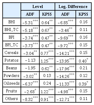
As the first step to investigate the lead-lag relationship between the agricultural import price and shipping freight rate, stationarity of time-series is examined. This is performed in two tests: ADF (Dickey and Fuller, 1981) with the null hypothesis ‘a time-series has a unit root and KPSS (Kwiatkowski et al., 1992) with the null hypothesis ‘a time-series is stationary’.

Table 2 presents the results of unit root tests. For the straight level, the null hypothesis of the ADF test is rejected at conventional significance levels in most cases (except for Potatos and Beans). However, the null hypothesis of the KPSS test is also rejected in most cases (see colums in ‘Level’), which indicates that it is uncertain that time-series in the dataset are stationary. Therefore, all the variables are differenced in logarithm and test results show that they become stationary (see columns in ‘Log. Difference’). Based on these results, all the time-series are estimated in VAR in terms of logarithmic difference in this study.

Table 2.

Results of Unit Root Tests

Table 3 shows the test statistics for AIC, which determines the optimal lag length in VAR estimations (i.e. i and j in Equation (1) and (2)). According to the rules of AIC, the lag with minimum value is selected for each pair of shipping freight rate and agricultural price.

Table 3.

AIC for Optimal Lag Order

Based on the results of unit root tests and AIC, Granger causality tests are performed. Table 4 reports the test results for spot freight rates (BHI and BPI). As seen, it is found that causality generally runs from the shipping freight rate to the price of agricultural produce. Specifically, for BHI, there is uni-directional causality running from shipping freight rate to Cereals, Potatos, Beans and Oilseeds. Bi-directional causality is found only for the pair of BHI and Fruits and there is no causality running from the agricultural price to the shipping freight rate.

Table 4.

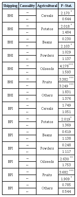
Results of Granger Causality Tests (Spot)

Similar results are reported for BPI (in Table 4), BHI_TC and BPI_TC (in Table 5). For these indices, uni-directional causality running from the shipping freight rate to the import price is found in Potatos and Oilseeds, while bi-directional causality is found in Fruits.

Table 5.

Results of Granger Causality Tests (Time-Charter)

5. Conclusions

This study investigates the lead-lag relationship between the shipping freight rate and the price of agricultural commodity imported into Korea. The results of Granger tests under the VAR estimation show the existence of causality running from the shipping price index to the commodity price supporting the previous finding that the shipping freight rate has a predictive power for future economic activity.

The finding in this paper offers several interesting implications. First, by examining the causal relationship between the shipping freight rate and the agricultural commodity price imported into Korea, this study augments previous research in the field of shipping transportation. In addition, Korean importers of agricultural produce can take advantage of information from the lead-lag relationship in their calculating and forecasting the import price and, ultimately, establishing corporate strategies.

Despite the important finding in the paper, there are still unfilled gaps that future research should focus on. Especially, further research efforts are needed for the variations in the import price by different commodity export countries. Moreover, the dataset on Korean-specific shipping freight rate or index can provide more detailed and interesting implications. Finally, empirical analysis can be augmented when controlled by other variables that possibly affect the demand (e.g. growth in population) and the supply (e.g. fluctuations in shipping tonnage) sides.

Acknowledgements

This work was supported by the 4th Maritime Port Logistics Training Project from the Ministry of Oceans and Fisheries and the Korea Maritime And Ocean University Research Fund.

References

1. Akaike H. 1974;“A New Look at the Statistical Model Identification”. IEEE Transactions on Automatic Control 19(6):716–723.

2. Bakshi G, Panayotov G, Skoulakis G. 2011. “The Baltic Dry Index as a Predictor of Global Stock Returns, Commodity Returns, and Global Economic Activity”. AFA Chicago Meetings Paper Proceedings

3. Bildirici M, Kayikci F, Onat IS. 2016;“BDI, Gold Price and Economic Growth”. Procedia Economics and Finance 38:280–286.

4. Dickey DA, Fuller WA. 1981;“Likelihood Ratio Statistics for Autoregressive Time Series with a Unit Root”. Econometrica 49(4):1057–1072.

5. Granger CW. 1969;“Investigating Causal Relations by Econometric Models and Cross-spectral Methods”. Econometrica 37(3):424–438.

6. Kavussanos MG, Visvikis ID, Dimitrakopoulos DN. 2010;“Information Linkage between Panamax Freight Derivatives and Commodity Derivatives Markets”. Maritime Economics and Logistics 12(1):91–110.

7. Kavussanos MG, Visvikis ID, Dimitrakopoulos DN. 2014;“Economic Spillovers between Related Derivatives Markets: The Case of Commodity and Freight Markets, Transportation Research Part E:”. Logistics and Transportation Review 68:79–102.

8. Kim CY, Park KS. 2019;“Lead-lag Relationship between Iimport Commodity Prices and Freight Rates: The Case of Raw Material Imports of Korea”. Journal of Korea Trade 23(2):34–45.

9. Kim CY, Shin Y. 2018;“A Study on the Use of Shipping Indices as Leading Indicators of International Trade of Korea”. Korea International Commerce Review 33(4):255–268.

10. Kim HH, Sung KD, Jeon JW, Yeo GT. 2016;“Analysis on the Relationship between Freight Index and Shipping Company’s Stock Price Index”. Journal of Digital Convergence 14(6):157–165.

11. Kim HS, Chang MH. 2017;“Analysis of the Synchronization between Global Dry Bulk Market and Chinese Container Market”. Journal of Navigation and Port Research 41(1):25–32.

12. Kim HS, Oh YS. 2012;“Empirical Approaches to Testing the Relationship between Stock Price and BDI”. Journal of Shipping and Logistics 75:687–702.

13. Kwiatkowski D, Phillips PC, Schmidt P, Shin Y. 1992;“Testing the Null Hypothesis of Stationarity against the Alternative of a Unit Root: How Sure Are We that Economic Time Series have a Unit Root?”. Journal of Econometrics 54(1–3):159–178.

14. Lee GU, Shin CH. 2019;“The Relationship Study for Major Petrochemical Complexes and Liquid Cargo Ports by the Granger and Toda-Yamamoto Causality Test”. Journal of Navigation and Port Research 43(6):469–474.

15. Lee SW, Kim JS. 2014;“An Analysis on Relationship between BDI and Financial Markets of Korea”. Journal of International Area Studies 18(1):181–200.

16. Sooriya B, Ryoo DK, Ahn KM. 2018;“Causal Relationship between Indian Ports’ Originated Container Traffic and Total Transshipments of Port of Colombo: A Granger Causality Analysis”. Journal of Navigation and Port Research 42(5):357–364.

17. Tsioumas V, Papadimitriou S. 2018;“The Dynamic Relationship between Freight Markets and Commodity Prices Revealed”. Maritime Economics and Logistics 20(4):267–279.

Article information Continued

This is an Open Access article distributed under the terms of the Creative Commons Attribution Non-Commercial License (http://creativecommons.org/licenses/by-nc/3.0/) which permits unrestricted non-commercial use, distribution, and reproduction in any medium, provided the original work is properly cited.

Fig. 1.

Food and Grain Self-Sufficiency Rates of Korea Source: Korea Rural Economics Institute

Table 1.

Descriptive Statistics for Variables

	Mean	Median	Max.	Min.	St. Dev.
BHI	565.24	521.48	1467.21	197.19	228.70
BHI_TC	8226.20	7625.19	21336.16	2363.84	3382.08
BPI	1320.05	1182.67	4304.90	324.19	734.66
BPI_TC	10552.56	9432.10	34592.47	2600.05	5930.55
Cereals	326.55	310.26	494.88	236.80	61.05
Potatos	514.80	472.75	983.00	252.26	159.37
Beans	556.93	523.22	803.61	425.93	90.00
Powders	626.95	634.56	725.07	479.07	55.50
Oilseeds	1030.47	1017.11	1596.60	653.89	168.43
Fruits	1506.59	1512.11	2243.25	804.84	315.24
Others	6579.21	6469.24	12290.08	3292.91	1661.75

Source : Baltic Exchange and KITA

Table 2.

Results of Unit Root Tests

	Level		Log. Difference
	ADF	KPSS	ADF	KPSS
BHI	−5.31^***	0.64^**	−6.85^***	0.16
BHI_TC	−5.18^***	0.67^**	−3.46^**	0.11
BPI	−3.74^***	0.47^**	−9.69^***	0.16
BPI_TC	−3.73^***	0.47^**	−9.72^***	0.15
Cereals	−3.04^**	0.77^***	−14.21^***	0.15
Potatos	−1.13	1.25^***	−13.95^***	0.40^*
Beans	−1.95	0.62^**	−17.96^***	0.21
Powders	−3.02^**	0.13	−14.26^***	0.12
Oilseeds	−6.37^***	0.24	−11.33^***	0.39^*
Fruits	−2.68^*	1.22^***	−4.98^***	0.15
Others	−8.32^***	0.91^***	−12.71^***	0.11

Note:

^{***, **, *}

denotes statistical significance at 1%, 5%, and 10% levels, respectively.

Table 3.

AIC for Optimal Lag Order

Shipping	Agri-cultural	Lag
Shipping	Agri-cultural	1	2	3	4	5	6
BHI	Cereals	−2.87	−2.90	−2.87	−2.90	−2.93*	−2.91
BHI	Potatos	−1.58	−1.72	−1.70	−1.82	−1.82	−1.82*
BHI	Beans	−3.31	−3.33	−3.32	−3.33*	−3.29	−3.26
BHI	Powders	−4.20	−4.24	−4.23	−4.25*	−4.22	−4.22
BHI	Oilseeds	−1.98	−2.08	−2.08	−2.17*	−2.13	−2.16
BHI	Fruits	−2.72	−2.79	−2.80	−2.86	−2.93	−2.99*
BHI	Others	−0.85	−0.93	−1.07	−1.06	−1.12*	−1.11
BPI	Cereals	−2.04	−2.07	−2.03	−1.98	−2.03	−2.07*
BPI	Potatos	−0.66	−0.79	−0.77	−0.80	−0.82	−0.92*
BPI	Beans	−2.45	−2.45*	−2.45	−2.41	−2.37	−2.43
BPI	Powders	−3.32	−3.35*	−3.33	−3.30	−3.27	−3.34
BPI	Oilseeds	−1.04	−1.17	−1.16	−1.17	−1.17	−1.25*
BPI	Fruits	−1.83	−1.87	−1.85	−1.87	−1.97	−2.09*
BPI	Others	−0.01	−0.08	−0.19	−0.15	−0.16	−0.25*
BHI_TC	Cereals	−2.69	−2.71	−2.69	−2.73	−2.76*	−2.75
BHI_TC	Potatos	−1.42	−1.55	−1.54	−1.67	−1.67	−1.69*
BHI_TC	Beans	−3.11	−3.13	−3.15	−3.16*	−3.12	−3.09
BHI_TC	Powders	−4.02	−4.05	−4.06	−4.08*	−4.05	−4.05
BHI_TC	Oilseeds	−1.76	−1.86	−1.88	−1.98	−1.94	−1.99*
BHI_TC	Fruits	−2.52	−2.59	−2.61	−2.66	−2.71	−2.77*
BHI_TC	Others	−0.65	−0.73	−0.89	−0.89	−0.95*	−0.94
BPI_TC	Cereals	−1.99	−2.02	−1.98	−1.94	−1.98	−2.03*
BPI_TC	Potatos	−0.62	−0.74	−0.73	−0.76	−0.79	−0.89*
BPI_TC	Beans	−2.40	−2.41	−2.41*	−2.37	−2.33	−2.39
BPI_TC	Powders	−3.28	−3.30	−3.29	−3.26	−3.23	−3.30*
BPI_TC	Oilseeds	−0.99	−1.12	−1.11	−1.13	−1.14	−1.22*
BPI_TC	Fruits	−1.78	−1.82	−1.81	−1.83	−1.92	−2.04*
BPI_TC	Others	0.03	−0.04	−0.15	−0.11	−0.11	−0.21*

Note:

indicates the lowest value in AIC.

Table 4.

Results of Granger Causality Tests (Spot)

Shipping	Causality	Agricultural	F-Stat.
BHI	→	Cereals	2.170 ^*
BHI	←	Cereals	0.644
BHI	→	Potatos	2.018 ^*
BHI	←	Potatos	1.484
BHI	→	Beans	0.230
BHI	←	Beans	2.103 ^*
BHI	→	Powders	1.029
BHI	←	Powders	1.137
BHI	→	Oilseeds	4.278^***
BHI	←	Oilseeds	1.593
BHI	→	Fruits	3.382 ^***
BHI	←	Fruits	3.249 ^***
BHI	→	Others	1.831
BHI	←	Others	1.376
BPI	→	Cereals	1.749
BPI	←	Cereals	1.051
BPI	→	Potatos	2.019^*
BPI	←	Potatos	1.369
BPI	→	Beans	0.619
BPI	←	Beans	1.138
BPI	→	Powders	0.248
BPI	←	Powders	1.117
BPI	→	Oilseeds	2.630 ^**
BPI	←	Oilseeds	1.753
BPI	→	Fruits	3.682 ^***
BPI	←	Fruits	1.909 ^*
BPI	→	Others	0.785
BPI	←	Others	0.544

Note:

^{***, **, *}

denotes statistical significance at 1%, 5%, and 10% levels, respectively.

^{→ and ←}

indicate the directions of causality.

Table 5.

Results of Granger Causality Tests (Time-Charter)

Shipping	Causality	Agricultural	F-Stat.
BHI_TC	→	Cereals	1.878
BHI_TC	←	Cereals	0.805
BHI_TC	→	Potatos	2.262 ^**
BHI_TC	←	Potatos	1.575
BHI_TC	→	Beans	0.332
BHI_TC	←	Beans	1.827
BHI_TC	→	Powders	1.186
BHI_TC	←	Powders	0.915
BHI_TC	→	Oilseeds	3.291 ^***
BHI_TC	←	Oilseeds	1.457
BHI_TC	→	Fruits	2.596 ^**
BHI_TC	←	Fruits	2.760 ^**
BHI_TC	→	Others	1.556
BHI_TC	←	Others	1.381
BPI_TC	→	Cereals	1.765
BPI_TC	←	Cereals	1.087
BPI_TC	→	Potatos	2.095 ^*
BPI_TC	←	Potatos	1.417
BPI_TC	→	Beans	1.293
BPI_TC	←	Beans	1.241
BPI_TC	→	Powders	0.818
BPI_TC	←	Powders	1.128
BPI_TC	→	Oilseeds	2.657 ^**
BPI_TC	←	Oilseeds	1.792
BPI_TC	→	Fruits	3.524 ^***
BPI_TC	←	Fruits	1.927 ^*
BPI_TC	→	Others	0.823
BPI_TC	←	Others	0.478

Note:

^{***, **, *}

denotes statistical significance at 1%, 5%, and 10% levels, respectively.

^{→ and ←}

indicate the directions of causality.