Effects of Macroeconomic Conditions and External Shocks for Port Business: Forecasting Cargo Throughput of Busan Port Using ARIMA and VEC Models
Article information
Abstract
The Port of Busan is currently ranked as the seventh largest container port worldwide in terms of cargo throughput. However, port competition in the Far-East region is fierce. The growth rate of container throughput handled by the port of Busan has recently slowed down. In this study, we analyzed how economic conditions and multiple external shocks could influence cargo throughput and identified potential implications for port business. The aim of this study was to build a model to accurately forecast port throughput using the ARIMA model, which could incorporate external socio-economic shocks, and the VEC model considering causal variables having long-term effects on transshipment cargo. Findings of this study suggest that there are three main areas affecting container throughput in the port of Busan, namely the Russia-Ukraine war, the increased competition for transshipment cargo of Chinese ports, and the weaker growth rate of the Korean economy. Based on the forecast, in order for the Port of the Port of Busan to continue to grow as a logistics hub in Northeast-Asia, policy intervention is necessary to diversify the demand for transshipment cargo and maximize benefits of planned infrastructural investments.
1. Introduction
The average annual growth rate in container handling volume in the Port of Busan was 6.0% from 2001 to 2008 (4.3% for imports and exports 8.3% for transshipment), and it has been steadily increasing. In the aftermath of the 2008 Financial Crisis and the bankruptcy of Hanjin, the average annual growth rate of the port stood at 4.3% between 2006 and 2021 (2.9% for imports and exports, and 5.9% for transshipment Moreover the average annual growth rate over the past five years (2016 through 2021) was dampened at just 3.1% (1.63% for imports and exports, 4.5% for transshipment Global container handling volume in 2021 stood at 265.8 million twenty-foot equivalent units (TEU), which represented an increase of 6.26% compared to the previous year. However, with 2,271 million TEU handled in 2021, Busan yielded a 2.26% lower than the global growth rate. The global average growth rate for container throughput had been 6.19% between 1996 and 2021, but the Port of Busan recorded a rate 6.81% over that same period, higher than the global rate. However, considering only a more recent period (2014–2021), the global average annual rate of fluctuation had been 3.31% while that of the Port of Busan had been 2.82%. There are several reasons for this trend: first, the slowdown in the economic growth rate of China as well as Japan and Korea (Drewry, 2021) which resulted in lower overall cargo volumes imported and exported. Second, the growth of container throughput in Chinese ports is a main contributor in the decline of transshipment cargo for the Port of Busan. In addition external economic shocks such as a sharp rise in oil prices due to the Russia-Ukraine War, is a another major threat to the container traffic volume in Busan. Therefore it is necessary to accurately estimate container traffic volumes in the Port of Busan in order to successfully develop strategic and investment policies.
Previous studies attempted to forecast cargo throughput using ARIMA-intervention model. In the case of Korea, Park(2021) forecasted the cargo throughput for Gwangyang Port utilizing an ARIMA model and OLS regression model including as variables government consumption, China’s imports and Korean exchange rate. Other studies showed the importance of including an economic shock into the model. For instance, Rashed et al. (2017) applied ARIMA and ARIMAX and incorporated in the model data post the 2008 financial crisis to forecast the cargo throughput of the port of an Antwerp. whilst Chung et al.(2009) investigated the financial crisis in the Chinese manufacturing industry. Lai et al.(2005) used ARIMA-intervention and included the September 11, 2001 shock.
Therefore, past literature showed the importance of including macro-economic factors and particularly external shocks as the financial crisis. Whilst the study considers general macro-economic variables the originality of the paper lies in incorporating the Russia-Ukraine War as an important model’s variable and other past economic shocks. The war has been an external shock that significantly disrupted supply chains worldwide and consequently ports’ cargo throughput. Hence, attempting to forecast ports’ cargo throughput under the current uncertainty can support ports’ managers and operators to cope with cargo volatility and improve decision-making in operations planning as well as investment strategies. The purpose of this study is to build a model that accurately forecast container throughput in the Port of Busan based on two existing models: the ARIMA (Autoregressive Integrated Moving Average) intervention model and the VEC (Vector Error Correction) model. Using univariate time-series methods, allow for forecasting times series models independent of other variables which are needed in multiple regression analysis and to capture long-time relationship amongst processes.
2. Theoretical background and Literature Review
2.1 Literature Review
In the study conducted by Park and Lee(2002), container traffic volume was estimated using a neural network back propagation learning algorithm in order to compensate for the shortcomings of existing statistical forecasting methods such as moving average, exponential smoothing and past time series data. This method shows the results of reducing forecasting errors by considering not only container traffic but also related economic variables such as the number of ships calls in the Port of Busan, cargo handling capacity, and income per capita as input variables.
Lai and Lu(2005) proposed a regression analysis for container traffic volume data on 18 different types of cargoes in the Port of Hong Kong over 17 years (from 1983 to 2000). Their study compared the predictive power of the method with an artificial neural network model.
Chung and Song(2007) compared the predictive power of a neural network model and a regression analysis model by selecting 10 major local cargoes traffic. The regression analysis was considered suitable for analyzing upward trends, and the neural network model was considered suitable for analyzing irregular and downward trends.
Kim(2008) estimated future container and cargo throughput of the Port of Gwangyang through a univariate time series model. This study also estimated container throughput by optimizing the analysis with the Winters additive model that considers trends and seasonal variations.
Shin, Kang et al.(2008) combined the ARIMA model and a neural network model to predict domestic container throughput and measure the suitability of the model combination, which has the strengths of both linear and non-linear models. This study demonstrated that the suitability of various models varies depending on intrinsic port characteristics and the predictive power of the models.
Lee and Ahn(2020) estimated container throughput based on the ARIMA method and own series data in previous studies. The work estimated locally-generated cargo throughput using the VAR model, and transshipment cargo was estimated using the VEC model.
This study uses the intervention-ARIMA model to supplement the previous studies and tests whether major external shocks, such as inancial crises, the bankrupcy of Hanjin and the Russia-Ukraine War have a significant effect on the container throughput for the Port of Busan, It is not necessary to separately estimate both locally-generated cargo and transshipment cargo as they have no significant differences from each other and they are both considered as cargo handled by the port. Therefore, this study uses, in a novel way, the VEC model to estimate combined local and transshipment cargo.
2.2 ARIMA & Intervention Models and VAR& VEC Models
Quantitative demand forecasting methods are largely divided into time series analyses and causal relationship analyses. ARIMA method, described by Box et al.(2015), is a time series analysis method based on univariate variables and is still used today as an analytical technique with excellent predictive power. However, this analysis method has a limitation as it is a univariate model that does not consider economic variables with close causal relationships. To overcome these challenges, this study analyzes the time series of casual variables as well as its own time series using multivariate models, including intervention, VAR and VEC models.
2.2.1 Intervention Model
Intervention factors analysis include factors affecting the time series due to external shocks such as changes in government policies, natural disasters, changes in consumption trends and in corporate strategy. In this study, relevant events include the Asian Financial Crisis of 1997, the energy crisis of the 1970s, the Global Financial Crisis of 2007–2008, the bankruptcy of Hanjin, and the Russia-Ukraine War. These factors have been considered as representative intervention factors affecting the container throughput of the Port of Busan. Such interventions can seriously alter the patterns within the time series. A factor that can affect the accuracy of estimated values calculated from a time series model is called an intervention (Glass, 1972).
Observation values at the time of intervention tend to have significantly larger or smaller values than those observed before the intervention. It is easy to find such observation values in an intuitive manner. Box and Tiao (1975) suggests an intervention model that is more realistic and can increase the accuracy of prediction by incorporating the influence of intervention factors in the model. Intervention in such models is often referred to as a dummy variable in general regression analysis.
2.2.2 VAR Model
The Vector Auto Regressive (VAR) Model serves as a powerful tool when two timeseries influence each other and each is expressed as a linear function of own past lags and other variables’ past lags. Hence, this model is a multivariate time series model that estimates the causal relationship between variables by combining the features of time series analysis and regression analysis. The VAR model, described by Sims (1980), does not distinguish between endogenous and exogenous variables, and it uses only time series information without considering restrictions of coefficient values.
This model is a useful technique to analyze the dynamic relationship between variables by estimating relations among all the variables of the time series without theoretical constraints. Its main advantage is its ability to make simple predictions without weighing the theoretical relationship between variables.
The VAR (p) model is a model that analyzes the characteristics and interrelationships of component variables by applying the AR model for a single variable to multiple variables. This model has the structure of the AR (p) model in which the vector xt is affected by past values during a period p. The model can be used for causal relationship analysis, impulse response analysis, and forecast error decomposition analysis.
The VAR model can analyze the causal relationship between variables through hypothesis testing on variable coefficients. For example, the model settings for the two variables Xt (GDP) and Yt (container traffic at the Port of Busan) are as follows:
First, regression analysis is performed on the past observations and constant terms of Xt and Yt, respectively. The causal relationship between X and Y is determined by estimating whether the coefficient of each variable is 0.
To test the hypothesis, this study uses the F-statistic or the W-statistic (Wald statistic) with an asymptotic distribution. This analysis method may have different values depending on the size of the considered lags. Therefore, in the empirical analysis, the appropriate balance can be found using the results of the Akaike Information Criterion (AIC) or the Schwarz Bayesian Criterion (SBC) analysis.
2.2.3 VEC model
In the VEC model, error (drift) refers to a state out of a certain plane of equilibrium, and correction indicates that this error returns to the equilibrium plane. If some non-stationary time series have a co-integration relationship, each unstable time series has a stationary relationship with a time series with a co-integration relationship. In other words, a linear relationship with such time series represents a long-term equilibrium relationship. This has the advantage of being able to analyze without stabilization (differential).
The following is a case where there is a cointegration relation (long-run equilibrium relationship) between the component variables of the vector time series yt consisting of n(4) variables: the container traffic in the Port of Busan, economic fluctuations, interest rates, and the economic size of China and the United States (GDP).
ρ: A coefficient that reflects the rate of recovery to the equilibrium point when it deviates from the long-term equilibrium relationship
∊i: Random error term
α: Cointegration vector defining long-run equilibrium relationship, Long-term relationship information between the component variables of the error correction term
3. Design of Study
3.1 Forecasting Container Traffic Volume in the Port of Busan using the Seasonal ARIMA Model
The target variable used in this study is the container throughput of the Port of Busan. Statistics of cargo throughput was retrieved from 96 separate monthly volumes published by the Korea Development Corporation from January 2014 to December 2021. The forecasting was performed by combining time series data of locally-generated cargo and transshipment cargo, as they are not significantly distinct1). This study uses Dickey-Fuller’s unit root test to determine whether a trend exists, and identifies the ARIMA model with AC and PAC tests. After that, it estimates container throughput by deriving an optimal prediction model through AIC and BIC values and error analysis.
3.2 Estimating using VAR and VEC Models
3.2.1 Endogenous Variable
The VAR model and the VEC model are techniques to analyze the dynamic relationship between economic variables by estimating the relationships among all available time series without considering economic theories. The VEC model is a valid analysis model when there is a certain trend (cointegration) relationship between variables, but it is difficult to process multiple variables. Therefore, this study includes different time series data related to the container throughput generated in the Port of Busan as endogenous variables. These variables include: the size of the Chinese economy (expressed in GDP), which is predicted to have the greatest impact on transshipment cargo volumes; Korea’s economic growth rate, which is most closely related to import/export cargo; a dummy variable represented by the economic crisis. Within the economic crisis, we considered three separate events such as 1) the global financial crisis 2) Hanjin bankruptcy and 3) the Russia-Ukraine war. However, for this last event, we considered as as important data, the ending part of 2021 as there were already signs of geo-political tension in the region and the market were starting to get affected by it.
Recent trends in container traffic volumes in the Port of Busan do not suggest much difference between locally-generated and transshipment cargo. Therefore, this study combines both of them and attempt estimating them. Container throughput is expected to have a long-term trend relationship with the size of the Chinese economy and Korea’s economic growth rate, for which the VEC model is well suited for an estimation. The endogenous variables of influence on container throughput were selected based on the results of previous studies and the Intelligence Network Data was collected by Clarksons for 128 months (January 2014 through 2021). More specifically, each variable was selected according to the following:
(1) Economic size and growth rate. Korea’s economic growth rate (gr_k) is a significant variable for locally-generated cargo, and the size of the Chinese economy (expressed in GDP) is a significant variable for transshipment cargo (Park, S. Y. and Lee, C. Y., 2002). According to the analysis, the size of the Chinese economy is more closely related to the transshipment cargo throughput of Busan port, rather than that of the world and the US economy.
(2) Economic crises. The study uses economic crises as a dummy variable, such as 1) the global financial crisis (value =1) 2) Hanjin bankruptcy(value =1) and 3) the Russia-Ukraine war(value =1) and the remaining time series periods (value= 0) (Shin, Park, and Lee, 2008).
3.2.2 Research Hypothesis
[Hypothesis 1] The size of the Chinese economy (GDP) has a positive effect on container throughput at the Port of Busan.
[Hypothesis 2] Korea’s economic growth rate has a positive effect on container throughput at the Port of Busan.
[Hypothesis 3] External events have a negative impact on container throughput at the Port of Busan.
4. Empirical Analysis
4.1 Results of Descriptive Statistical Analysis
Table 1 shows the statistics of the selecetd variables, including the container throughput for the Port of Busan, which is considered a dependent variable. During the study period, 96 months of data are used to verify the empirical model.

Descriptive statistics for variables
(unit; teu, 10million$)
As shown in Table 2, the average monthly container throughput in the Port of Busan is 1,731,404 TEU. According to Lee and Ahn (2020), this volume is higher than the average volume of 1,682,441 TEU for the period from 2014 to 2019. However, the monthly average local cargo volume has increased from 817,407 TEU to 905,293 TEU, but transshipment cargo fell, from 863,831 TEU to 825,259 TEU.

Correlations analysis
Table 2 shows the correlation coefficients between the selected variables. Both locally-generated and transshipment cargo were found to have a significant correlation with the size of the Korean and Chinese economies. However, Korea’s economic growth rate does not appear to have a significant influence. Analysing the data from 2014 to 2019, the correlation coefficient of transshipment cargo with China’s GDP decreased from 0.863 to 0.475, confirming that the relative dependence on China is overall decreasing. The correlation coefficient of locally-generated increased slightly, from 0.617 to 0.62. According to the data from 2014 to 2019, the correlation coefficient of locally-generated cargo with Korea’s GDP increased from 0.628 to 0.755, and the correlation coefficient of transshipment cargo decreased, from 0.767 to 0.577.
4.2 Forecasting with Seasonal ARIMA Model
In this section, we apply a seasonal ARIMA model due to the seasonality of container throuhput shown by the port of Busan over the years. Table 3 shows the results of the unit root test (Dickey-Fuller test) to test whether time series data of variables exhibit a trend. According to the test results, unlike in the past, there is no trend in the locally-generated cargo volume of the Port of Busan but there is a slight trend in the transshipment cargo volume. Therefore, this study integrates locally-generated cargo and transshipment cargo into Busan total container throughput (bteu) and estimates it without any difference. As a result of calculating the lag by ACt and PAC analysis using the container throughput (bteu) variable, three seasonal models are made as follows: arima bteu, ma(1) sarima (1,1,0,12), arima bteu, ar(1) ma(1) sarima(1,1,0,12), arima bteu, ar(2) ma(1) sarima(1,1,0,12). As a result of testing the three models aic, bic, RMSE, and R2, the optimal models were selected as seasonal models such as arima bteu, ar(2) ma(1) sarima(1,1,0,12). Table 4 shows the results of the analysis.

Dickey-Fuller test Results

ARIMA model(bteu) analysis results
As shown in Table 5, the AR(2), MA(1) seasonal model has the least AIC and BIC, and the AR(2)MA(1) seasonal model has the largest R2, which describes the likelihood (LL) and attests to the explanatory power of the model. Looking at the root mean squared error (RMSE) of the four models in Table 6, the AR(2) MA(1) seasonal model has show the smallest error, so it is selected as the optimal model. Therefore, this study forecast the container throughput of the Port of Busan based on the optimal model.

Statistics of RMSE

ARIMA_Intervention Model analysis results
Table 6 describes the analysis results by adding the intervention variable (X) to the AR(2)MA(1) seasonal model, which is the optimal predictive model. According to the analysis results, the X dummy variables representing external shocks (financial crises, Hanjin bankruptcy and the Russia-Ukraine War) have considerable effects yielding a significance level of 1%. The regression coefficient is equal to −65759.52, showing a negative (−) effect on the container throughput of the Port of Busan.
Y = Port of Busan Container Traffic Time Series Data (January 2014 to December 2021) and X = Intervention Variable
4.3 Influencing Factor Analysis and Prediction by VEC Model
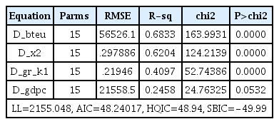
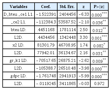
The influencing factors of the container throughput at the Port of Busan shown in Table 7 are as follow: economic fluctuations, Korea’s economic growth rate, and the size of the Chinese economy. Unlike in the past, the size of the Korean economy and the US economy in GDP are not considered as significant variables, and they have a multicollinearity problem with the size of the Chinese economy in GDP, which has the greatest impact on the container traffic volume. For this reason, they were excluded from the analysis. According to the result of the DF unit root test, the container throughput (bteu), economic fluctuations (X), Korea’s economic growth rate (gr_k) and the size of the Chinese economy (GDP) are endogenous variables with trends (cointegration). Therefore, this study tests the relationship among these variables using the VEC model. In the first stage, when the lag is determined by the indicators (AIC, HQIC and SBIC), the optimal lag is shown as lag 1 and lag 4. According to the results of vecrank analysis shown in Table 8, the optimal number of ranks is two. That is, there are two cointegration relationships between endogenous variables. Therefore, Tables 8 and 9 show the results of VEC model analysis with 4 lags and 2 ranks.

AIC. HQIC. SBIC results

Johansen tests for cointegration
Fitness of Variables
Looking at R2 values, which describe the explanatory power of endogenous variables in Table 10, own time series of the container throughput (bteu) is the largest, at 0.6833, followed by economic fluctuations (x) at 0.6204, Korea’s economic growth rate (gr_k), and China’s GDP (gdpc).
VEC Analysis Results
According to the analysis results of the VEC model shown in Table 10, cointegration 1 (D_bteu _ce1 L1) shows a long-run equilibrium at 1% significance level, and cointegration 2 (D_bteu _ce2 L1) indicates a long-run equilibrium at 5% significance level. The economic fluctuations factor (X), an external shock and Korea’s economic growth rate have a significant effect on the container traffic volume at lag 1 and lag 2. The size of the Chinese economy has a significant effect only at lag 1.
In the first cointegration (ce1) of Table 11, the economic fluctuations factor (X) is negligibly small, so the causal relationship between the coefficients is expressed as follows: bteu = 1,540,517 + 43913.75 gr_k + 0.7446215 gdpc. In other words, the container throughput (bteu) increases by 43,913.75 of Korea’s economic growth rate and is positively related to 0.746215 of China’s GDP. In the second cointegration (ce2), the causal relationship between the coefficients is meaningless because neither Korea’s economic growth rate nor China’s GDP were verified as significant variables.
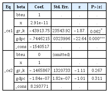
Johansen Normalization Analysis Results
Table 12 shows the results of estimating container throughput in 2022 using the seasonal ARIMA seasonal model and the VEC model (the causal relationship model).

Forecasting Comparison between ARIMA and VEC
The annual forecast of the seasonal ARIMA model based on its own time series data is 22,906,584 TEU in 2022. The VEC model, which considers economic fluctuations (external shocks), Korea’s economic growth rate, and China’s GDP as well as its own time series, is estimated to be 23,300,956 TEU.
4.4 Results of Impulse Response Analysis
The following figures show the results of the impulse response function analysis of the impact of China’s economic size (gdpc), Korea’s economic growth rate (gr_k), and economic fluctuations (X2) on the container throughput (bteul) for six steps. The top left diagram shows the effect of the Chinese economy on the container throughput of Busan port. At first, the effect is large in magnitude (a deecrease and then an immediate steady increase) but then it shows a a more stagnating pattern. On the top right, the diagram shows that the influence of previous Chinese economy on the size of Chinese economy is almost unchanged.
The mid raw diagram shows the effect of the Korea’s economic growth rate on the container throughput of Busan port. There is a trend showing a generalized increase but then it shows a decreasing one indicating that the economic growth rate of Korea has limited effect on the Busan port’s container throughput. The diagram on the right confirms that the Korean economic growth has almost no effect on the size of the Chinese economy.
The bottom diagram shows the impulse response of economic fluctuations on Busan port container throughput. It shows an initial downwards trend until step three and then it slightly increases just above zero and stagnates. On the right side diagram, the econoimc fluctuations have almost no effect on the Chinese economy.

Response for bteu by gdpc, gr_k, X2
5. Conclusion
Recently, the increase in the container throughput of the Port of Busan has slowed considerably. From 2016, the rate of increase in volume started to slow compared to the global container volumes. Container volume in Busan accounted for 11.6% of global container traffic in 2015, but fell to 11% in 2021. In order to optimize the scale of new port facilities set to be built, it is important to accurately determine whether this slowdown is a temporary trend or a structural and long-term problem.
First, according to the results of this study, transshipment cargo, which leads the increase in the container traffic volume, has a correlation coefficient with China’s GDP of 0.863 in 2019, but just 0.475 in 2021. This indicates that the growth of transshipment cargo from China has slowed significantly, to the extent that trade dependence on China has decreased significantly.
Second, local cargo has became more dependent on China, but China’s economic growth rate slowed to an unprecendeted level.
Third, the correlation coefficient of locally-generated cargo with Korea’s GDP was 0.628 from 2014 to 2019, but increased to 0.755 by the end of 2021. The correlation coefficient of transshipment cargo decreased from 0.767 to 0.577.
Fourth, since the increase in transshipment cargo volume has slowed, it is possible to additionally estimate the total cargo volume when estimating the container handling volume of the Port of Busan. Therefore, this study considers economic fluctuations taking into account China’s GDP, Korea’s economic growth rate and external factors as endogenous variables and estimates their effects on container volume using the VEC model.
Since China’s GDP is still the biggest factor influencing container traffic volume, it is pivotal to attempt formulating a strategy aimed at attracting transshipment cargo from China. Since economic fluctuations have a negative (−) effect, it is necessary to establish strategies and systems to appropriately mitigate external shocks and economic fluctuations and respond to them. Therefore, the study findings can support both Busan Port Authority (BPA) and container terminals’ managers in operational strategies and investments decision-makings. In particular, retaining transshipment cargo from and to China is fundamental and the proposed forecast of this study can contribute managers’ strategic decisions. Further, the study’s findings are important for ports’ managers in order to know when an external shock has an impact on cargo throughput and when not. This has several implications in relation to the responsiveness time needed, magnitude and effects on operations’ continuity and more generally on business performance and employment. With these results in hand, port managers’ can react comprehensively to a macroeconomic shock knowing the effect it will have on the port’s container throughput.
However, this study has several limitations. First, prediction errors were reduced by reinforcing data with causality through time series. Second, the study did not make any mid to long-terms predictions which could be helpful for port managers to support stategic and investment in a longer time horizon. Furthermore, future research should attempt comparing container throughput at the Port of Busan and the throughput of other competing ports in the Far-East region.
Notes
https://sin.clarksons.net(as of April 12, 2022)