A Basic Study on Connected Ship Navigation System

2.1 Communication network

Communication network must be constructed first to design the system, because the slave ship needs to receive position data from the master ship wirelessly to set the route. The transmission control protocol / internet protocol (TCP/IP) socket communication method was used in this study. Fig. 1 shows the communication procedure of the system, the master ship is the server and the slave ship is the client.

Fig. 1

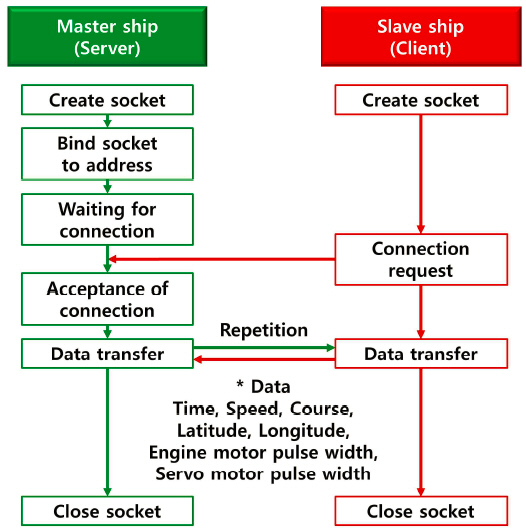
TCP/IP socket communication procedure

The communication procedure is as follows. First, the server and client create sockets. The server binds the IP address and port number to the created socket, then waits for the client to connect. If the client requests a connection to the server, then the server receives the request and accepts the connection. Once connected, the two ships exchange data with each other such as time, speed, course, latitude, longitude, engine motor pulse width and rudder servo motor pulse width. These data are used for the slave ship to set up the route. When the master ship determines that it is no longer necessary to transmit data, the socket is closed to terminate the connection.

2.2 Route planning algorithms

When the slave ship successfully receives the data, the slave ship stores the latitude and longitude of the master ship as a reference point. Then the slave ship calculates the course and distance to the reference point using middle latitude sailing method. If the calculated distance is 5 m or less, the slave ship is considered to have already passed the reference point, and the distance and course to the next reference point are calculated. This process is repeated when the slave ship is underway.

Middle latitude sailing method is based on the assumption that “the departure(p) between two specific points is equal to the arc length of the meridians of the two points at the middle latitude(L_m).”. If the middle latitude is less than 60 ° and the sailing distance(D ) is within 600 nautical miles, the error range is less than 1%.(Yoon et al., 2013).

When the starting point is A (L₁,λ₁) and the arriving point is Z (L₂,λ₂) , the course(C ) and the sailing distance (D) between the two points are calculated by Eq. (1) and Eq. (2).

Where difference of longitude DL_o, difference of latitude l, middle latitude L_m and departure p are obtained by the following equations.

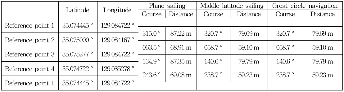
Table 1 shows the results of calculating the course and distance between each reference point using the plane sailing method, middle latitude sailing method and great circle navigation method.

Table 1

Comparison of plane sailing method, middle latitude sailing method and great circle navigation method.

Although the distance between the reference points is less than 80 m, there was a difference between the plane sailing method and middle latitude sailing method about 5 to 6 degrees on the course and about 34 m on the total distance. Since the plane sailing method assumes the earth as a plane, the theoretical error is large. On the other hand, the calculation results of the middle latitude sailing and the great circle navigation method were almost same. Because the great circle navigation method has high accuracy. But, it has a large amount of calculation and has the disadvantage that the ship’s course should be changed frequently. So, simple calculation but high accuracy middle latitude sailing method was adopted in this study.

2.3 Automatic steering controller

(a) Ship manoeuvring motion model

Considering the ship as a rigid body, the ship manoeuvring motion is described for the ship fixed coordinate system(G-xyz) with the coordinate origin at the ship’s center of gravity(G) as shown in Fig. 2.

Fig. 2

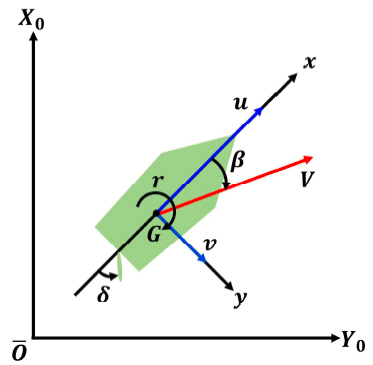
Ship fixed coordinate system

Where δ is rudder angle, β is drift angle, r is turning rate, u and υ are x-axis speed and y-axis speed, and V is the sum of u and υ. And the ship manoeuvring motion can be formulated as a combined motion by the inertia, propulsion and external forces. On the other hand, the mathematical model proposed by Nomoto et al.(1957) is relatively simple and has the advantage that the slave ship manoeuvring motion could be expressed as a relationship between input(rudder angle) and output(turning rate), not in terms of fluid force. Nomoto model has limitations in representing the motion of the ship accurately. However, the purpose of this paper is to find out the effectiveness of the proposed system using RC boats, so simple Nomoto model was adopted that can predict the manoeuvring motion model of ship with minimal information. And the autoregressive with exogenous variables(ARX) model(Ljung, 1987) was used to estimate the manoeuvring indices K and T, unknown coefficients of Nomoto model. The ARX model generates a transfer function from input-output data, and then estimates the parameters of the transfer function. This method has been used in a study by Kim(2011) to build the USV manoeuvring motion model.

(d) PD controller

Generally, proportional-derivative(PD) controllers or proportional-integral-derivative(PID) controllers are widely used for steering of model ship. By the way, PD controllers have characteristics that the overshoot is smaller and the settling time is shorter than PID controllers(Lee et al., 1985). So, PD control was adopted to design the automatic steering system. Fig. 3 shows the process of a digital PD controller. Where, K_P is proportional gain, T_D is derivative time, T_f is derivative time constant and T_s is sampling time.

Fig. 3

Block diagram of digital PD controller

The designed controller of the slave ship repeatedly performs the following actions to follow the target course. First, calculates the error(e (z)) by comparing the target course(ψ_r) and the current course(ψ). Then, control variable(u(z)) is calculated by the proportional-derivative actions. The control variable(u(z)) is limited to –35 to 35 degrees(u_s (z)) by the saturator and entered into the ship manoeuvring motion model. Finally, the ship manoeuvring motion model outputs the turning rate(r), which changes the current course(ψ).

In addition, a first-order low-pass filter is applied as in Eq. (13) to prevent derivative kick caused by high frequency noise in derivative action.

(13) 2TD(z−1)(Ts+2Tf)(Ts−2Tf)

where

(14) Tf=TDN

Here, N is a coefficient for adjusting the bandwidth of the filter, and usually has a value between 8 and 20(Åström & Hägglund, 1995). It was set to 10 in this study.

To find the optimal values of parameters K_P and T_D of the digital PD controller, the relay feedback tuning method(Åström & Hägglund, 1984) was used. This method generates critical oscillation using a transport delay and a relay with an amplitude of d. Fig. 4 shows the process of the relay feedback tuning method.

Fig. 4

Block diagram of relay feedback tuning method

From the critical oscillation graph, the critical period(T_c) and amplitude(a) could be found, and then the critical gain (K_c) is calculated by Eq. (15).

(15) Kc=4dπa

The parameters K_P and T_D of the PD controller is calculated by Eq. (16) and Eq. (17) using the Ziegler-Nichols tuning method(Ziegler & Nichols, 1942).

(16) KP=0.8Kc

(17) TD=Tc/8

2.4 Speed controller

When the slave ship follows the master ship, the distance between the two ships should be kept constant for safety and communication stability. However, it is difficult to keep the speed constant even though the revolutions per minute(RPM) is kept constant, because the experimental boats are small as about 1 m and are easily affected by waves and winds. So, the speed controller was designed to keep the slave ship from 7 m to 12 m from the master ship.

Fig. 5 shows the flowchart of the slave ship speed controller. The distance between two ships(D_s) is calculated by the positions of the master ship(L₁ , λ₁) and the slave ship(L₂, λ₂) using middle latitude sailing method. Then, the controller changes the motor pulse width(P_m) according to the distance(D_s). The pulse width controls the motor RPM of the slave ship.

Fig. 5

Flowchart of slave ship speed controller

3.1 Experimental setup

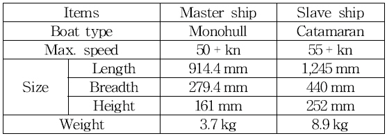
To verify the mathematical model of ship manoeuvring motion and the proposed system, sea experiments were conducted with two remodeled RC boats as shown in Fig. 6. The detailed specifications of the two boats are given in Table 2.

Fig. 6

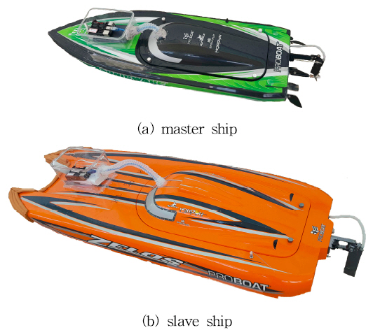
Experimental boats

Table 2

Specifications of boats

The systems of both boats are identical. Each boat had a propulsion system consisting of an electronic speed controller, brushless DC motor and propeller, and a steering system comprised of a servo motor and rudder. Both systems were controlled by pulse width modulation with a frequency of 50 Hz. To control the entire system, a microcontroller Arduino Uno and a microcomputer Raspberry Pi 3 Model B+ were equipped on the boat. These devices also performed boat-to-boat communications, sensor data collections, and route planning algorithms. Finally, a GPS sensor to measure the position of the boat and an radio frequency(RF) receiver to receive signals from a RF remote controller were equipped.

The experiments were conducted on the waters near Korea Maritime and Ocean University as shown in Fig. 7.

Fig. 7

Experimental site

3.2 System identification results

The experiment was conducted as a turning test to estimate the orders(n_a, n_b) and parameters(ana , bnb ) of the ARX model by analyzing rudder angles(δ) and turning rates(r). During the experiments, the Beaufort scale was 2 and the average wind speed was 2.2 m/s. But small wavelets on the surface were occurred due to the current to the south. Fig. 8 and Fig. 9 shows the experimental scene and the trajectory of the slave boat. The average speed of the slave boat was 6.0 kn(3.1 m/s).

Fig. 8

Experimental scene for system identification

Fig. 9

Trajectory of slave ship

The orders and parameters of the ARX model were determined using MATLAB system identification toolbox. The orders of the model were determined as n_a = 6 and n_b = 6 using FPE criterion, and the corresponding parameters ana and bnb were determined by the least square method.

Fig. 10 shows the turning rates obtained from the sea experiment(r) and calculated by the ARX model(r_A). The coefficient of determination R² of the obtained ARX model is about 0.9387, which means that the ARX model and the slave ship manoeuvring motion have a significance of about 94%.

Fig. 10

Turning rate by sea trial(r) and ARX model(r_A )

To obtain the PD controller parameters K_P and T_D , the relay feedback tuning method was used. Adding a relay with an amplitude(d) of 10 and a transport delay of 1 second to the slave ship manoeuvring motion model, a critical oscillation graph with an amplitude(a) of 16.60 and a critical period(T_c) of 8 is generated as shown in Fig. 11.

Fig. 11

Critical oscillation graph

The critical gain(K_c) was calculated by Eq. (15) as 0.767. The parameters of PD controller were calculated by Eq. (16) and Eq. (17) as K_P = 0.614 and T_D = 1.000. In sea experiment, K_P and T_D are tuned a little to prevent overshoot.

3.3 System verification results

The experiment was conducted to confirm that the slave ship autonomously follows the route of the master ship when the master ship is navigated manually. During the experiments, the Beaufort scale was 2 and the average wind speed was 1.8 m/s. But small wavelets on the surface were occurred due to the current to the southwest. Fig. 12 shows the experimental scene at sea. The average speed of the slave ship was 7.2 kn(3.7 m/s) and the master ship was 6.2 kn(3.2 m/s).

Fig. 12

Experimental scene for system verification

Fig. 13 shows that the slave ship autonomously follows the route of the master ship at a certain distance. The green and red lines represent each trajectory of the master ship and the slave ship. And the time indicated by the arrow shows the moment that the boat has passed through that position. The average speed of the master ship was 7.2 kn(3.7 m/s) and the slave ship was 6.2 kn(3.2 m/s).

Fig. 13

Trajectories of master ship and slave ship

Fig. 14 shows the rudder angle and motor pulse width of the slave ship. The slave ship continuously used the rudder to follow the route of master ship. And the motor pulse width was autonomously changed to maintain a constant distance from the master ship.

Fig. 14

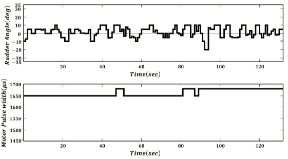
Rudder angle and motor pulse width of slave ship