Analysis of Stem Wave due to Long Breakwaters at the Entrance Channel

Article information

Abstract

1. Introduction

Recently, large scale harbor structures at deep water area are increasing to meet the necessary water depth for mooring basin and approaching waterway to meet the trend of very large ship. Most of harbor structures such as berth, protective jetty or breakwater of a navigable inlet are having vertical shape to keep the economic construction feasibility. These types contribute to the future port expansion because they are easy to couple with the existing harbor structures. Meanwhile, there are many investigations on progressive wave to grasp the safety of vertical structures but few of wave transformation studies causing wave height amplification due to the existing of these structures at a coastal inlet or harbor entrance. Among these large vertical structures, the breakwater at deeper zone is usually being constructed in a long detached manner and therefore, in addition to the incident and reflected waves, there appears a stem wave propagating along the wall, where the angle of incidence β is defined as the angle between the normal to the wave crest and the vertical wall as shown in Fig. 1 Generally, the height of the stem wave increases as the wave travels along the wall and the width of the stem wave extends progressively. Once the stem wave develops, the wave overtopping amount will be increased and it brings stability problem of bottom blocks. Furthermore, it impacts to ship navigation near the shore structure and might cause erosion of coastal bottom and failure of the structure. Therefore, it might need to analyze the character of stem wave by interpretation on interaction of wave and structure for consideration of structure crest height and impact to wave fields.

Fig. 1

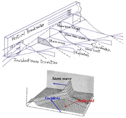
Sketch of stem wave development along vertical wall

Since the stem wave pattern was first found by Perroud (1957) from the laboratory experiments for the reflection of solitary waves from a vertical wall, some experimental results on the stem wave were shown together with numerical analysis. Among them, Mase et al. (2002) gave the results for stem waves along vertical wall due to random wave incidence, especially made stem wave characteristics comparison of regular wave and irregular wave response, including development of stem wave and impact from breaking wave. Yoo et al. (2010) had shown that the size of stem wave in the tangential direction of the vertical wall increases depending on the increase of incidence wave angle to the wall without any relation to regular or irregular wave. However, it was found that the nonlinearity of incident wave reduces the stem wave height and breaking wave constrains the grown of stem wave. Although those studies by Park et al. (2003), Lee & Yoon (2006), and Lee et al. (2007) have shown similar results by Mase et al. (2002), the engineering interests on numerical model application to the real fields are still low. In this study we will discuss in detail the impact of irregularity and nonlinearity to stem wave development and apply numerical models to the long vertical breakwaters along the coastal waters.

2. Basic Equation for Numerical Model

The governing equations for numerical models to analyze the stem wave in this study are based on two groups. One is a regular wave form which is linear elliptic approximation with nonlinear dispersion relationship and another is an irregular wave form which is nonlinear Boussinesq approximation with linear dispersion relationship. First, the extended mild slope equation can be obtained from original mild slope equation (Berkhoff, 1972) by allowing slow modulation of waves in the direction of wave crests. It simulates the combined effects of wave refraction-diffraction and also includes the effects of wave dissipation by bottom friction, breaking, nonlinear amplitude dispersion, and harbor entrance losses. The basic equation may be written as Equation (1):

where η^(x, y) (x, y) = complex surface elevation function, from which the wave height can be estimated, wave frequency under consideration (in radians/second), (x,y) are the horizontal coordinates, C (x, y) = phase velocity = σ/k, C g (x, y) = group velocity = ∂σ/∂k = nC with σ² = gktanh(kd), k(x, y) = wave number (= 2π/L) with the wave length(L), related to the local depth d(x, y) through the linear dispersion relation: n = {1 + 2kd/(sinh2kd)}/2, w = friction factor, and γ = a wave breaking parameter. We have used the following form of the damping factor, following Dalrymple et al. (1984).

where a(= H/2) is the wave amplitude: wave height(H ), and f_r is a friction coefficient. Typically, values for f_r are in the same range as for Manning’s dissipation coefficient ‘n’, specified as a function of (x, y) assigning larger values for elements near harbor entrances to consider entrance loss. For the wave breaking parameter γ, we use the following formulation (Dally et al., 1985; Demirbilek, 1994).

In addition to the above relationships, simulation of nonlinear waves may be conducted by using the mild slope equation. This is accomplished by incorporating amplitude-dependent wave dispersion, which has been shown to be important in certain situations. Equation (4) is rearranged to include the nonlinear dispersion relation used in place of Equation (1).

where

F1={cosh(4kd)−2tanh2(kd)}/8sinh4(kd),

F2={(kd)/sinh(kd)}4.

Along the open boundary where outgoing waves must propagate to infinity, the Sommerfeld radiation condition applies

where the scattered wave potential η^s=∑n=0∞Hn(kr), as shown in Mei (1983), where Hn are the Hankel functions of the first kind. Applying above equation to the governing equation and after proper assembling through Galerkin finite element formulation with boundary conditions, finally we come to the general form of linear algebraic equation as [A]{η^}={f}. In order to solve the extended elliptic mild slope equation, the problem has to be solved simultaneously over the entire domain. We used iterative methods from studies of Panchang et al. (1991) and Li (1994) for the present study.

The second model is the Boussinesq wave model. The depth integrated the continuity equation and momentum equation developed by Nwougu(1993) which is applied to shallow water up to the deep water limit h/L = 0.5) but considering steep near breaking waves in shallow water, Nwougu(1996) had modified those in fully nonlinear form as shown here. We are going to use the modified equation for numerical analysis.

where, η is the water surface elevation, u_f is the volume flux density of horizontal velocity ∫−hηudz, h is the water depth, u_α is the horizontal velocity at z = z_α, zα=−0.535h→zα+h=0.465(h+η), g is the gravitational acceleration, and the operator ∇=(∂/∂x, ∂/∂y). A fully nonlinear equation for the volume flux density u_f is revised by equation (8).

The effect of energy dissipation due to a turbulent boundary layer at the seabed has been modeled by adding a bottom shear stress term to the right hand side of the momentum equation u_α. Here f_w at equation (9) is the wave friction factor. The linear dispersion relation of the Boussnisesq model is given by the phase speed as shown in equation (10) and those parameters were depicted from Nwogu & Demirbilek(2001).

where

3. Model Evaluation

3.1. Model Specification

For evaluation of numerical model, it was referred to hydraulic model experiment result. Hydraulic model investigation of the Mach reflection for obliquely incident regular and irregular waves was done for a rectangular basin with a vertical breakwater by Lee and Yoon (2006). Mach reflection by obliquely incident wave smaller than a critical angle might develop the stem wave. Table 1 shows the experimental conditions under both regular wave and irregular wave for the evolutions of stem waves. The height of the breakwater is high enough for waves not allowing wave overtopping. Wave generators were installed at the bottom side of the wave basin and wave absorbers at the top side as shown in Fig. 2. Various incident wave directions were used in the experiment.

Table 1

Hydraulic model experiment conditions under regular wave and irregular wave

Fig. 2

Experimental setup for constant water depth(after Lee & Yoon, 2006)

The numerical mesh and grids for the given domain and other simulation conditions are summarized in Table 2.

Table 2

Experimental conditions for numerical models

The regular model contains 115,549 nodes and irregular model has 151,200 grids. The element and grid space are 15m and 10m, respectively. Wave periods were 9s and 9.1s and wave heights were 3m and 3.4m.

3.2. Model Evaluation

Fig. 4 and Fig. 5 compare the numerical and experimental results of the cases for random waves with those for monochromatic waves with both models with respect to the result of hydraulic model experiment (Lee & Yoon, 2006). They also compared numerical result with linear parabolic wave model with both linear and nonlinear dispersion relationship. The relative stem wave heights along the wall in Fig. 4 are distributed for the different incident angles. Horizontal axis indicates the relative distance with respect to wave length. All the cases show good agreement between hydraulic model result and numerical model result. The difference of the stem wave amplification along the vertical breakwater is not significant. Although regular wave model gives close response to the hydraulic experiment result, the response show undulation, whereas the Boussinesq model shows smooth response.

Fig. 4

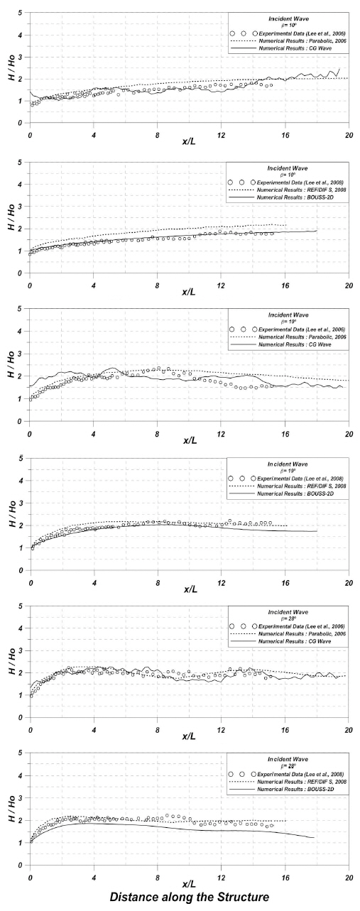
Comparison of normalized wave heights along the breakwater(x) from regular and irregular wave models

Fig. 5

Comparison of normalized wave heights perpendicular to the breakwater(y) from regular and irregular wave models

The stem wave height increases at early stage but becomes stable after about 8 wave length away from the structure tip. As the incident wave angles to the vertical breakwater become large, the normalized stem wave heights become large and the nonlinearity of the incident waves reduces the stem wave height. Fig. 5 shows comparisons of the distributions of wave amplification in the normal direction to the vertical wall. The stem waves due to the regular model show the pattern of standing wave as the incident angle increases, while Boussinesq model reduces this pattern due to the irregular wave nature. However, regardless of the nonlinearity of incident waves, the width of stem waves shows almost the same. The width of stem waves is defined by the distance from the wall to the closest point of a small wave height as shown in Fig. 5. With the incident angle β=10°, the width of stem wave is about twice of the wave length, whereas β=19° gives a half of this. Although stem wave patterns are different between regular wave model and Boussinesq model in the direction of normal to the vertical wall, the stem wave widths from both models are quite similar. Present study suggests that Boussinesq model is a good tool for the analysis of the stem wave in real field as the following field application.

4. Field Application

4.1. Model Formulation for Serial Breakwaters

For field application of the stem wave analysis, we surveyed field conditions where there is a series of very long breakwaters in the east coast of Korea. The considered port is a newly expanded and strategically important port for domestic base industries both electricity and gas by handling coals and LNG. The berthing facilities are protected by two detached breakwaters, which are parallel to coastline, having 900m and 1,800m of length as shown in Fig. 3. Table 3 shows the numerical formulation and wave input condition and the grid size to meet the required resolution as 6 to 12 elements per wave length. Four event waves from KMA offshore wave records(2015-2016) at Donghae and Uljin, which might cause stem waves near the breakwaters depending on the locations under extra ordinary sea state, were selected. First two waves are traveling from the north to south during winter and rest two are on summer, vice versa.

Fig. 3

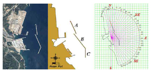
Location map and incident wave directions

Table 3

Summary of numerical input and model formulation

4.2. Field Stem Wave Response Analysis

Fig. 6 and Fig. 7 shows contour plots of the wave response near the breakwaters for both Ho=3.0m, T=10.9sec, β=13° from north and Ho=3.0m, T=10.9sec, β=20° from south byboth models. Here Ho denotes incident wave height from offshore. They presents the wave height distributions. The standing wave pattern of stem wave for regular model shows clearly, while the pattern is not represented in irregular wave model, especially from the south. Because of serial breakwaters, the gap between breakwaters and aligned angle cause more complicate stem wave generation. Although the clear development of stem wave pattern does not appear, it is observed a secondary stem wave form through the breakwater gap. The finding means that there might be a possible stem wave development at the lee side of breakwaters through the gap depending on the incident wave direction. This impact should be included in the analysis of the basin tranquility near the berthing area and vessel traffic near these breakwaters.

Fig. 6

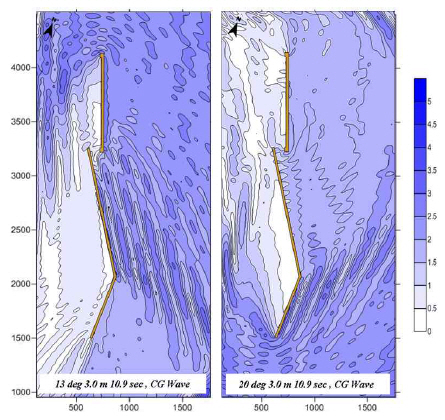
Contour plots of water surface elevations for both H=3.0m, T=10.9sec, β=13° and H=3.0m, T=10.9sec, β=20° by CG Wave model

Fig. 7

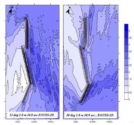
Contour plots of water surface elevations for both H=3.0m, T=10.9sec, β=13° and H=3.0m, T=10.9sec, β=20° by BOUSS-2D model

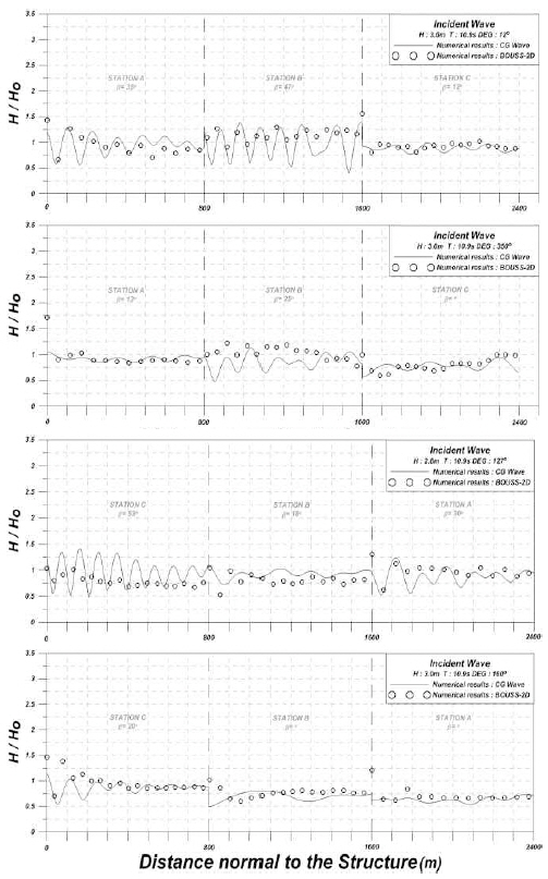
Both Fig. 8 and Fig. 9 show comparison of numerical model results in terms of responses along and normal to the serial breakwaters, respectively. The vertical dashed lines with stations A, B, and C show separation of breakwaters. β is the incident wave angle to each breakwater section.

Fig. 8

Comparison of normalized wave heights along the serial breakwaters

Fig. 9

Comparison of normalized wave heights perpendicular to the serial breakwaters

Because slit and semi-circled caisson breakwaters were adopted here, the reflection coefficient 0.5 was introduced here. Due to serial breakwaters the development of stem wave shows complicate near the connection point. Although the response was reduced, the general pattern shows similar as previously compared at the verification. Fig. 10 shows the normalized wave heights of parallel and normal to the serial breakwaters for four incident wave directions. Left graphs show the normalized wave height along the breakwaters and right graphs show those perpendicular to the breakwaters. Both models show similar pattern but the nonlinear Boussinesq model results shows higher response, except for incident waves from south. That’s because of the alignment of serial breakwaters. South breakwater blocks out incident waves to the north breakwaters and shows flat pattern.

Fig. 10

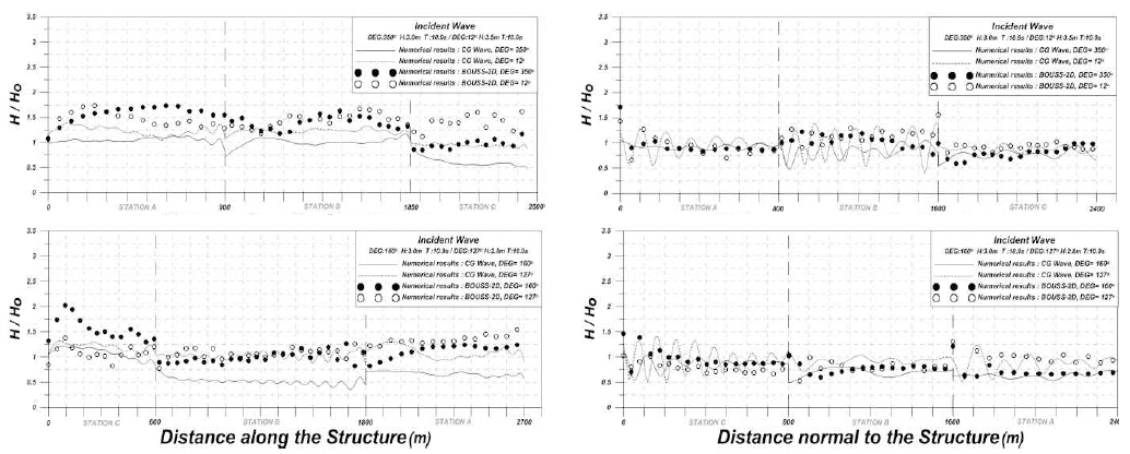
Comparison of normalized wave heights along and perpendicular to the serial breakwaters for various incident wave directions

5. Results and Discussions

The present study investigated the impact of irregularity and nonlinearity to stem wave development from waves obliquely propagating to the long vertical breakwaters at the coastal waters by numerical simulation using linear elliptic approximation with nonlinear dispersion relationship and nonlinear Boussinesq approximation with linear dispersion relationship. The summary of the results are as follows:

Article information Continued