A Study of Optimization of α - β - γ - η Filter for Tracking a High Dynamic Target

Article information

Abstract

1. Introduction

Tracking filters are the essential part of target tracking as they play the key role of tracking error reduction and making accurate estimations. The α - β and α - β - γ filters, which are steady state Kalman filters for tracking constant velocity and constant acceleration targets respectively, are limited in their capacity to follow a high maneuvering target, defined by a jerky motion, with good accuracy. The jerky motion is reduced considerably when the target tracking equations are modelled to make provision for a constant jerk. The third order α - β - γ filter, therefore, becomes a fourth-order filter when the design is extended to include the constant jerk parameter.

Several approaches have been introduced recently in an attempt to design filtering equations that model for the constant jerk. They have been found to out-perform the constant acceleration α - β - γ filter in terms of error reduction and ability to follow a maneuvering target with jerky movements. Mehrotra (1997) suggested a jerk model for tracking highly maneuvering targets marred by unexpected changes in the speed. The simulation results indicate better performance of the jerk model than that of the lower order filters. The study undertaken by Chen (2008) also showed an improvement in the target tracking accuracy when the α - β - γ - σ filter was utilized in tracking a constant jerk model compared to the conventional α - β - γ filter. Similarly, Seyyed (2009) designed the steady state Kalman filter α - β - γ - η, an extension of the α - β - γ filter, for tracking high maneuvering target and concluded that compared to the standard α - β - γ filter, the new design was more superior in terms of ability to follow a jerky model with a good accuracy.

Wu (2011) went further and proposed an evolutionary programming based on α - β - γ - σ filter that provided an optimal simulation technique for a maneuvering target with jerky movement. In addition, with highly accurate and efficient prediction of the target trajectory, this new fourth-order filter was associated with a reduced computational time. In Wu's research, estimation factors were given by corresponding intervals and the parameters were determined by Taguchi method, which was complex and needed lots of computations. Incidentally, the mathematic model of estimation has a mistake in Equation 6 and 7 in this paper, the numbers 2 and 6 should be contained in the denominator.

The series of filter optimization researches were started by Jeong(2015), since then the filter optimization work was focused on the optimization of correction parameters. Njonjo (2016a) investigated the performance of the fading memory α - β - γ filter on a high dynamic target warship. The research concluded that the filter was capable of tracking the highly maneuvering vessel with a relatively good accuracy in terms of noise reduction. Njonjo (2016b) also indicated that the fading memory algorithm had better performance in numbers of α - β - γ filter algorithms. This research was further extended by Pan (2016) where the filter was optimized in order to improve its tracking ability by reducing the noise to a minimum. The optimization procedure involved varying the value of the discounting factor, ξ, with the residual error and determining the ξ that corresponds to the minimum error. The study demonstrated that the optimal filter uniquely varies with the initial speed and average speed of the target under consideration.

The investigation presented in this study is aimed at improving the accuracy of the jerky motion of a high maneuvering target. The design examined is a fourth-order α - β - γ - η filter using the fading memory filter algorithm which is easier to control and has less computations compared with other methods mentioned above. The filter is first optimized, then its performance is compared with that of the optimal memory α - β - γ filter as further discussed by Pan (2016) based on its ability to follow the jerky motion with a higher order of accuracy.

2. α - β - γ- η Filter Model

The α - β - γ - η filter is a constant gain, fourth-order tracking filter. The four state vector includes position, velocity, acceleration and jerk, a time derivative of acceleration. The jerk is modelled as a constant and includes zero mean white Gaussian noise.

Based on the two major stages of α - β - γ filter algorithm which were illustrated by Mahafza et al. (2004), the prediction stage and smoothing stage can be derived as equations 1-8. Equations 1-4 are the prediction equations for position, velocity, acceleration and jerk respectively where they are updated from the estimated state thereby lowering the tracking error Equations 5-8 are the smoothing equations which are computed by adding a weighted difference between the observed and the predicted position to the forecast state.

Prediction;

Smoothing;

Where;

The filter weight constants, α , β, γ and η, are computed by the fading memory filter algorithm as shown in Equations 9-12 and are extracted from Brookner (1998). The ξ represents the discounting factor that minimizes the least squares error for a constant jerk input model of target dynamics. The smoothing constants are determined from the value of the discounting factor hence the optimization of the filter is applied on the ξ as illustrated by Pan (2016).

3. Simulation of α - β - γ - η Filter

A target model vessel on motion with the initial relative velocity of 50.4　m/s and at the initial position (573, 1038.4) on the Cartesian coordinates as observed from the radar range measurements from own ship was considered for simulation. The sample measurements were collected at the time interval of three seconds which corresponds to the radar scan rate of 20 rev per minute. Table 1 below shows a summary of the initial input in generating the original target motion.

Table 1

Target’s initial conditions

3.1. Input motion model of the target dynamics

The model equations used in generation of the original target motion are as shown in Equations 13 & 14.

(13) Xi=a[10 sin(1.2wi)]+7cos(0.99wi)+8sin(0.7wi)+6 cos(2wi)+9 sin(3wi)+5 cos(3wi)+10i,

(14) Yi=b[20 cos(0.3wi)+22 sin(2wi)].

The resulting data was then sampled at intervals of 3 seconds to give the true trajectory of the target as shown below in Fig. 1.

Fig. 1

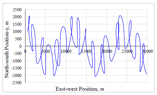
Target’s true position

3.2. Noise addition

Since the measurements from the radar sensor contain errors, this was taken into account by adding a zero mean random white Gaussian noise with a standard deviation, σ, of 10 m to the true position sample. This error distribution in the observation is as shown in Fig. 2 and Fig. 3.

Fig. 2

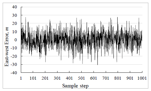
East-west error in the observation

Fig. 3

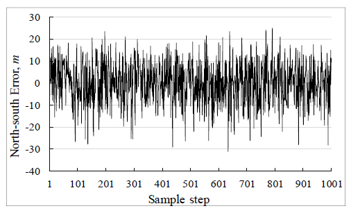
North-south error in the observation

3.3. Determination of optimal ksi, ξ

The filter weight constants α , β , γ and η values depend on the value of the discounting factor, ξ as shown in Equations 9-12. Therefore, in order to obtain the optimal smoothing coefficients, optimization of the critically damped filter focusses on adjusting the ξ value experimentally through trial and error method.

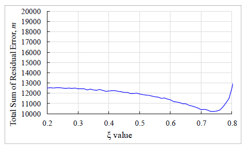
The process of optimization begins by computation of the total transient error which is the sum of the squares of the difference between the true trajectory and the predicted trajectory. The purpose of the optimization is to find the discounting factor that minimizes this error then to use this information to compute the optimal smoothing constants. This is, therefore, achieved by plotting a range of the discounting factor, which lies in the interval [0, 1] and with a step increase of 0.01, against the corresponding transient error. Thirty simulation tests are then carried out for each ξ and the average obtained. The resulting figure is as shown in Fig.4 below. According to this graph, the value of ξ corresponding to the least residual error is 0.74. Fig. 5 and 6 serve to show the consistency regarding the optimal ξ and therefore uphold the validity of the results as they both indicate a similar value of the optimal discounting factor. They represent plots of the total error difference between the true and smoothed trajectories and between the observed and predicted trajectories respectively against corresponding ξ values.

Fig. 4

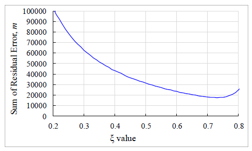
Average summation of the error difference between true and predicted positions against corresponding value of the discounting factor, ξ for 30 simulations

Fig. 5

Average summation of the error difference between true and smoothed positions against corresponding value of the discounting factor, ξ for 30 simulations

Fig. 6

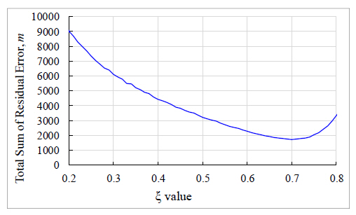
Average summation of the error difference between observed and predicted positions against corresponding value of the discounting factor, ξ for 30 simulations

4. Performance of the Filter

The performance of the optimal α - β - γ - η filter is evaluated based on its ability to follow the maneuvering target with ease and with an increased reduction of overshooting along the prediction trajectory due to jerky movements. In addition, the filter’s performance is further investigated based on its capability of reduction of tracking error. The performance is then compared with that of the optimal α - β - γ filter under similar conditions of target motion.

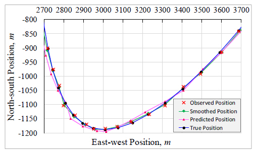
Using the obtained optimal discounting factor (ξ=0.74) the optimal filter weights were computed and consequently the predicted and smoothed trajectory were obtained. Fig. 7 shows the true, observed, predicted and smoothed trajectories of α - β - γ - η filter. The curve enclosed in the rectangle is enlarged for clearer viewing as shown in Fig. 8. The positional trajectories obtained from simulation tests carried out under similar conditions using the optimal α - β - γ filter are as shown below in Fig. 9. From the obtained trajectories, the α - β - γ - η filter can be observed to easily follow the highly maneuvering target with greater sensitivity as indicated by the steadiness in the predicted and smoothed trajectories. In contrast, the predicted and smoothed trajectories resulting from the α - β - γ filter are seen to have erratic changes and overshooting at various points on the trajectories indicating the filter’s inability to respond well to random changes in speed and quick maneuvers particularly for this type of trajectory.

Fig. 7

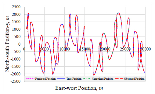
Target’s true, observed, predicted and smoothed position, α - β - γ - η filter (optimal ξ=0.74)

Fig. 8

Enlarged view of target’s true, observed, predicted and smoothed position corresponding to Fig.7

Fig. 9

Target’s true, observed, predicted and smoothed position (ξ=0.64), α - β - γ filter

Fig. 10 and Fig 11 plot the tracking error and estimation error of α - β - γ - η filter and α - β - γ filter. It is clear that the two filters perform good in tracking high dynamic motion. However, after carefully comparing the tracking error of them, the α - β - γ - η filter performs better than α - β - γ filter.

Fig. 10

Tracking error and estimation error of α - β - γ - η filter

Fig. 11

Tracking error and estimation error of α - β - γ filter

After comparing the tracking result of two filters, it is visibly clear that after optimization the α - β - γ - η filter has a higher performance than the α - β - γ filter. Quantitatively, the total tracking error and total estimation error are used to evaluate the performance of two filters. As shown in the table below, the α - β - γ filter demonstrates the best performance when ξ=0.64 with the total tracking error amounting to 19,592.20 m. On the contrary, when ξ=0.74 the α - β - γ - η filter depicts its optimal performance with total tracking error resulting to 17,858.93 m . The accuracy in tracking is therefore improved by 1,733.27 m equivalent to 8.9% higher. Similarly, the estimation accuracy is increased by 419.49 m on employing the α - β - γ - η filter. Meanwhile, the standard deviation of tracking error and estimation error of α - β - γ - η filter are a little smaller than α - β - γ filter, it indicates that the stability of fourth-order α - β - γ - η filter is higher than that of α - β - γ filter.

Table 2

Summary of the total tracking and estimation accuracy obtained from the optimal filters

5. Conclusion

Target motions defined by high maneuvering and jerky movements such as high dynamic vessels require prompt and accurate predictions of the target dynamics. Standard filters such as the α - β - γ filter are incapable of tracking the randomly changing accelerations with good accuracy since they are designed to track constant acceleration motions only. Therefore, a higher order steady state filter is required to take care of the jerky maneuvers.

The results obtained from simulation tests of the high dynamic target model indicate a better performance of the jerk model filter in terms of ability to follow the maneuvering target with a greater sensitivity compared to the α - β - γ filter under the same operating conditions of target motion. This attribute is due to the inclusion of the jerk smoothing constant which is responsible for taking care of the sudden changes in acceleration and target maneuvers. In addition, the tracking accuracy increased by 8.9% for the jerk filter model compared to the α - β - γ filter model. Meanwhile, the stability of fourth-order α - β - γ - η filter is higher than that of α - β - γ filter.

In this study, a theoretical model was adopted to generate the target’s dynamics with the case which was simulated by trigonometric equations. The authors intend to apply the results of this study to much more theoretical cases and real situation in the near future in order to test the effectiveness of the proposed algorithm.

Article information Continued