Tropospheric Anomaly Detection in Multi-reference Stations Environment during Localized Atmosphere Conditions-(1) : Basic Concept of Anomaly Detection Algorithm
Article information
Abstract
Extreme tropospheric anomalies such as typhoons or regional torrential rain can degrade positioning accuracy of the GPS signal. It becomes one of the main error terms affecting high-precision positioning solutions in network RTK. This paper proposed a detection algorithm to be used during atmospheric anomalies in order to detect the tropospheric irregularities that can degrade the quality of correction data due to network errors caused by inhomogeneous atmospheric conditions between multi-reference stations. It uses an atmospheric grid that consists of four meteorological stations and estimates the troposphere zenith total delay difference at a low performance point in an atmospheric grid. AWS (automatic weather station) meteorological data can be applied to the proposed tropospheric anomaly detection algorithm when there are different atmospheric conditions between the stations. The concept of probability density distribution of the delta troposphere slant delay was proposed for the threshold determination.
1. Introduction
The GPS (Global Positioning System) signal is vulnerable to the environment that the signal passes through. It is known that the troposphere delay is one of the largest limiting factors for precise positioning. A localized or regional troposphere anomaly, which is an extremely localized weather condition or inhomogeneous atmospheric condition, can corrupt an entire network solution in a network RTK (Real-Time Kinematic)(Kim, 2012). Such an imbalanced network error can effect on the other network solutions or rover solutions including maritime DGPS(Ahn, 2006; Ahn, 2007; Seo, 2009; Shin, 2013). There have been several studies on how to detect GNSS faults and improve the positioning performance for DGPS applications(Cho, 2007; Kim, 2010; Zhang, 2005; Zheng, 2004). The network errors caused by localized troposphere anomaly can degrade the correction message to the rover. Thus, finding out whether there is an inhomogeneous weather condition or not between reference stations in a network RTK environment is needed.
Troposphere error has dry and wet delays. The dry delay accounts for 90 % of the troposphere delay. The troposphere dry delay can be well predicted, whereas the troposphere wet delay highly depends on the weather conditions, especially the water vapor component such as precipitation(Ahn, 2007). For the prediction of troposphere zenith total delay, the position data such as height and latitude of the rover or reference stations are needed with the meteorological data of pressure, temperature and vapor pressure(Saastamoinen, 1972). Then, the troposphere slant delay can be estimated by using the mapping function according to satellite elevation(Niell, 1996). If it is assumed that the network has enough short baseline, the tropospheric delay at the rover position would be similar because the weather conditions at the rover position also would be similar with the reference stations. However, predicting the tropospheric delay at the rover position when the baseline becomes longer is needed(Han, 2014).
This paper proposes a detection algorithm for tropospheric anomalies and anomalous satellites that can degrade the correction message quality in use of reference station networks. This algorithm uses the multi-meteorological stations’ data in a network RTK concept when there is a localized troposphere anomaly around certain reference stations. In an atmospheric grid constituting four meteorological stations, the low performance point (LPP), which is the farthest position (or the most ambiguous position) from the four stations can be found because it is assumed that the weather conditions at LPP would not be the most difficult to predict well. If there is no tropospheric anomaly between stations then, the troposphere zenith total delay (ZTD) is similar at the four meteorological stations. However, the troposphere ZTD would be different at each station when there is a severe tropospheric anomaly at a local station. If the troposphere ZTD difference between stations has larger than usual value (earned by statistical data), it is known that there is the tropospheric anomaly between stations that can cause a degradation of correction data. Then it is possible to detect the anomalous satellites having nonlinearity of ZTD at a LPP.
For the threshold determination to detect an anomalous satellite during localized atmosphere conditions that can cause the tropospheric delay irregularities, the probability density function of delta slant delay between stations was proposed.
2. Tropospheric anomaly detection algorithm
2.1 Detection algorithm concept
Korea meteorological administration (KMA) has over 500 automatic weather stations (AWS) shown in Fig. 1, and it provides meteorological data as an on-line service(KMA, 2012).

Automatic water stations (AWS) of Korea Meteorological Administration (KMA)
One atmospheric grid needs three meteorological stations at least three stations, but it considers four stations that consist of one atmospheric grid. If the grid size is smaller, it is better to collect the meteorological data to estimate more accurate troposphere zenith total delay (ZTD) at a low performance point (LPP), which is the farthest point from all the stations assumed to be the most ambiguous point in the grid. If each reference station’s (RS’s) earth-centered earth-fixed (ECEF) coordinates are (x1, x2, …, xn), (y1, y2, …, yn), (z1, z2, …, zn), respectively, LPP can be estimated as Eq. 1.
Fig. 2 shows one atmospheric grid that consisted of four meteorological stations. There are six cases (six lines, 4C2) to connect the two stations among the four stations. Then, it is possible to calculate the foot of the perpendicular from the LPP to the six lines. Two meteorological stations (RS1 and RS2 in Fig. 3) can be selected, which have a minimum value to the foot of the perpendicular. This has the most linearized formation from the two stations to a LPP. If the atmosphere conditions are similar at the selected two stations then, the difference in the troposphere ZTD between RS1 and RS2 would be similar. Linearized ZTD at LPP can be estimated from the geometric formation from RS1, RS2 to the LPP positions in proportion to the distance as shown in Fig. 3. Troposphere ZTD can be estimated as in Eq. 2,

Delta troposphere ZTD from common satellites between RSs in multi-reference stations environment
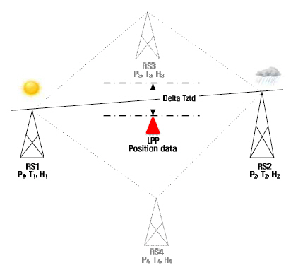
Delta troposphere ZTD estimation at LPP during localized troposphere conditions in an atmospheric grid
Saastamoinen zenith hydrostatic delay (ZHD) and zenith wet delay (ZWD) are as follows(Saastamoinen, 1972; Misra, 2006).
here, P0 is the total surface pressure [hPa], e0 is the partial water surface pressure [hPa], T0 is the surface temperature [K], ϕ is the latitude [deg] and H is the height of the sensor [km]. Partial water surface pressure e0 can be estimated as follows,
here, HR is the relative humidity [%], Pws is the water vapor saturation pressure [Pa]. Pws is as follows,
here, e is the constant of 2.718.
If the elevation angle E [deg] is applied to ZTD, slant delay (SD) can be estimated as follows,
The mapping function mi(E) at a specific elevation E can be presented as f(E , ai, bi, ci) and i can be marked as d for the hydrostatic mapping function, and w for the wet mapping function(Herring, 1992).
In Eq. (11), the hydrostatic mapping function needs a correction term for the height difference of the observation site, and the correction term for the height is as follows,
here, H is the height of the site [km], and the coefficients of correction terms aht, bht, cht are given as constants(Niell, 1996).
The delta troposphere ZTD (hereafter denotated as delta Tztd or ΔTztd ) is the difference of the estimated troposphere ZTD (hereafter denotated as eTztd) and calculated troposphere ZTD (hereafter denotated as cTztd) at the LPP. eTztd is earned by linearization of Tztd1,2 at RS1 and RS2 because eTztd at the LPP can be estimated by linearity according to the distance d1 (from RS1 to LPP) and d2 (from RS2 to LPP).
cTztd at LPP is calculated using RS1 and RS2’ meteorological parameters with the position data of the LPP. If there is no local atmospheric anomaly between RS1 and RS2 then, the calculated Tztd1 (cTztd1) using RS1’s meteorological parameter P1, T1, H1 is similar to the calculated Tztd2 (cTztd2) using RS2’s meteorological parameter P2, T2, H2 at the LPP (P: pressure, T: temperature, H: humidity). However, if there is a localized atmosphere anomaly such as a typhoon or regional torrential rain etc., cTztd1 and cTztd2 would not be different at the LPP due to the different atmosphere conditions at RS1 and RS2. The larger difference with eTztd and cTztd1,2 which can cause a larger error is defined as delta Tztd as shown in Fig. 3.
cTztd
1 =
cTztd
2 =
The delta troposphere SD (hereafter denotated as delta Tsd or ΔTsd ) applying elevation angle at the LPP can be estimated using a mapping function to ΔTsd of Eq. 8, and is as follows,
Here, the mapping function of the delta Tztd to the delta Tsd is simplified using the hydrostatic delay mapping function in Eq. 8.
Finally, the anomaly flag is generated according to the delta Tsd results. If the delta Tsd is larger than the threshold (here, it can be set based on the statistical results described in section 2.3) then, the flag is ‘1’, otherwise the flag is ‘0’.
2.2 Detection algorithm flow
The detection algorithm flow of a tropospheric anomaly in multi-reference stations environment is shown in Fig. 4.

Anomaly detection algorithm flow during localized troposphere conditions using atmospheric grid in multi-reference stations environment
Block A collects the meteorological data of P, T, and H at meteorological reference stations in Fig. 4. Then the delta Tztd at the LPP is estimated in block B. From the delta Tztd in block B, delta Tsd is calculated using a mapping function. In the anomaly detection block, the calculated delta SD in block B is compared to threshold and the anomaly flag is generated in Fig. 5.
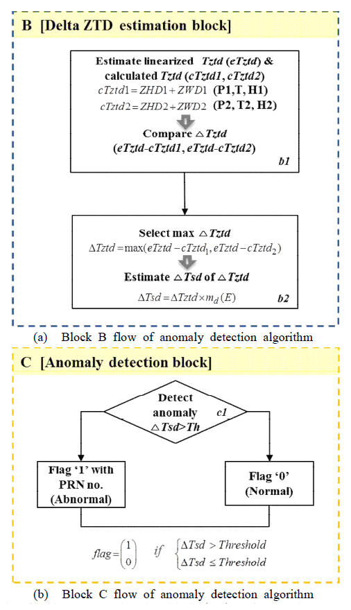
Delta ZTD estimation block (top) and anomaly detection block (bottom)
2.3 Threshold determination
For the detection of anomalous satellites during localized atmosphere environment, threshold determination problem can be critical to discriminate an anomalous satellite in network RTK environment. The normalized probability density function can be used for the threshold determination problem using statistical data during a certain period. In the final step of anomaly detection algorithm, the delta Tsd can be compared to the threshold. Then, the statistical delta Tsd can provide a critical value for the threshold. A random variable X is normally distributed with mean μ and variance σ2 if its probability density function (pdf) is as follows(Ribeiro, 2004),
here, x is the delta Tsd, μ is the mean value of delta Tsd and σ2 is the variance of delta Tsd, respectively.
For the threshold determination, σ can be used (σ is the square-root of the variance known as standard deviation).
Given a real number
Then, the probability that a Gaussian random variable lies in an interval whose width is related with the standard deviation is as follows.
The threshold value can be determined within 1σ ~ 3σ according to the threshold level of detection algorithm. It is considered that the delta Tztd and Tsd are Gaussian distributed if there was no tropospheric delay irregularity between RSs in an atmospheric grid.
Fig. 6 shows an example of delta ionospheric slant delay probability density distribution with 3σ threshold having a similar concept with the delta tropospheric slant delay in network RTK environment(Yoo, 2011).

Concept of threshold determination using the probability density distribution during localized atmosphere anomaly
Statistical value of atmospheric parameters of AWSs in an atmospheric grid can be used to derive more reliable threshold determination during a lone period.
3. Conclusions
Localized weather conditions regarding inhomogeneous atmosphere environment can corrupt network solutions in network RTK and can affect other network solutions through imbalanced network errors. It can also cause the degradation of the correction message quality in multi-reference stations environment. Therefore, implementing a monitoring technique during localized troposphere anomaly is needed.
This paper proposed a detection algorithm concept for the tropospheric anomalies during localized atmosphere conditions using the multi-meteorological stations’ data. An atmospheric grid consisting of four stations can find out a LPP (Low Performance Point) that is assumed as the most ambiguous point from known positions of meteorological stations. It is possible to find two linearized stations that form the most linearity from the position of the LPP. The troposphere ZTD (Zenith Total Delay) would be similar at the two selected stations, which are RS1 and RS2, if the tropospheric conditions are similar at RS1 and RS2. However, the troposphere zenith total delay has a large difference between the two stations if the weather conditions are severely different at the two stations. The detection algorithm for tropospheric anomalies uses the delta troposphere SD projected the delta troposphere ZTD between stations to an elevation at the LPP. If the delta troposphere SD is larger than the, the detection algorithm generates an anomaly flag of ‘1’.
The concept of threshold determination using the probability density function of the delta slant delay was proposed. Statistical results using the atmospheric parameters can provide the threshold value according to the detection level
To evaluate the proposed detection algorithm, it is needed that apply the meteorological data of AWSs in an atmospheric grid to the proposed algorithm and analyze the results for further study.