A Basic Study on Development of a Tracking Module for ARPA system for Use on High Dynamic Warships
Article information
Abstract
The maritime industry is expanding at an alarming rate hence there is a perpetual need to improve situation awareness in the maritime environment using new and emerging technology. Tracking is one of the numerous ways of enhancing situation awareness by providing information that may be useful to the operator. The tracking module designed herein comprises determining existing states of high dynamic target warship, state prediction and state compensation due to random noise. This is achieved by first analyzing the process of tracking followed by design of a tracking algorithm that uses α – β – γ tracking filter under a random noise. The algorithm involves initializing the state parameters which include position, velocity, acceleration and the course. This is then followed by state prediction at each time interval. A weighted difference of the observed and predicted state values at the nth observation is added to the predicted state to obtain the smoothed (filtered) state. This estimation is subsequently employed to determine the predicted state in the next radar scan. The filtering coefficients α, β and γ are determined from a pre- determined value of the damping parameter, ξ. The smoothed, predicted and the observed positions are used to compute the twice distance root mean square (2drms) error as a measure of the ability of the tracking module to manage the noise to acceptable levels.
1 Introduction
Tracking is defined as the continuous computation and updating of the various parameters which are essential to be known by the operator(Burger, 1983). A tracking filter estimates the true values of the ship’s movement that is position and speed, based on radar measurements of the ship’s location. The goal of the filter is to reduce the effect of the noise generation on the measurement and improve the stability of the system. The α – β – γ tracking filter is a third order special case of the Kalman filter that utilizes the tracking error, also known as innovation, to predict the next position. However the performance of the filter mainly relies upon the smoothing parameters α , β and γ(Benedict et al, 1962).
A high dynamic warship is characterized by high velocity, acceleration and high maneuvering in the face of oncoming threats. Therefore, it is of great importance that an elaborate system is put in place to track and predict the next state in quick successions. The α – β – γ filter is easy to design and implement. In addition, it is designed to track quick maneuvering vessels or vessels that undergo constant acceleration, a property the α – β filter has limited capability.
Numerous α – β – γ filter algorithms have been designed for application in tracking and for system optimization. However, only a few have designed systems with optimum damping parameters. Kalata(1984) suggested the tracking index in an attempt to characterize the behavior of the filter and hence obtain optimal set of the smoothing parameters. Tenne et al(2002) analyzed the performance characteristics of the α – β – γ filter.
Development of a tracking module can be approached in two different perspectives;
Own ship remains stationary while target ship moves at high speed.
Both own ship and target move at high speed.
This paper focuses on the first viewpoint whereby own ship is at a fixed point as a basic study of development of a tracking module and feasibility of application of α – β – γ filter to a high dynamic motion. The tracking algorithm utilizes the α – β – γ filter to track the motion of a high dynamic target warship advancing at a very high speed as observed from own ship which remains stationary. Prediction of the target’s state is made based on the smoothed estimates of the target’s present state. The radar scan rate is set at 20 rpm which is considerably high hence the tracking interval time is 3 seconds for every scan. All predicted and smoothed (corrected) positions are linked to the observed positions with twice root mean square distances (2drms) and comparison is made between a scenario with random gaussian noise and one without noise. The smoothing error and the prediction error are computed for each case and then compared to determine how the process noise influences the accuracy in prediction.
2 Design of the α – β – γ tracking filter
The α – β – γ filter follows inputs of state variables such as position, velocity and acceleration. The acceleration is assumed to be constant and without steady state errors. It is a steady state Kalman filter which assumes a third order model and produces better estimates of position, velocity and acceleration for the nth observation. Smoothing is important for error reduction in the predicted states which is achieved by adding a weighted difference between the observed and the predicted position to the forecast position as shown below in Eqs. (1)~(3). Eq. (4) is the prediction equation where the predicted position is computed from values obtained after smoothing(Mahafza et al, 2004).
Where; the subscripts o, p and s denote the observed, predicted and smoothed state parameters respectively.
P , V and a are the position, velocity and the acceleration respectively;
t is the simulation time interval;
n is the number of steps;
The smoothing parameters α , β, and γ are computed as shown in Eqs. (5)~(7)(Mahafza et al, 2004).
Where ξ is the damping parameter whose range is in the interval 0 ≤ ξ ≤ 1. When ξ = 1, no smoothing is present as all the smoothing coefficients are equal to zero. Similarly, for ξ = 0, heavy smoothing occurs.
3 Simulation
3.1 Initial Values
The initial relative speed of the target ship was 50 m/s and the course over ground was 0450. The radar scan rate was set at 20 rpm hence the image refreshed every 3 seconds. The target ship was tracked for total time duration of about 8 hours and 20 minutes since the number of points were 10, 000. Table 1 shows a summary of the initial state of the high dynamic target warship.

Input Parameters
3.2 Equations of Target’s Motion
The target motion model was as follows;
where the subscripts t and 0 denote the true and initial state values respectively.
X , V and A are the target’s position, velocity and acceleration matrices.
3.3 Noise Generation
The assumption is that tracking is influenced by random disturbances or process noise. Therefore, the algorithm employed in this tracking module utilizes the Matlab’s function ‘normrnd.m’ to generate Gaussian white noise with a mean of 50m/s and 45° for relative speed and course respectively and a variance of σ2 = 22.
3.3 The Tracking Process
The tracking process involves obtaining initial states of the target acquired from observation of the radar measurements. However, in this study the observation was a random value generated on Matlab. Based on these initial values the next state was predicted. The α – β – γ filter was then applied to compute the smoothed estimates by adding a weighted difference between the observed and the predicted position to the predicted state as shown in Eqs. (1)~(3). The smoothed estimate was then used to predict the next state using Eq. (4). This cycle of prediction and filtering to obtain smoothed estimates was repeated for the whole duration of the tracking period.
4 Simulation Results and Analysis
In order to evaluate the performance of the α – β – γ filter algorithm, the simulation tests were performed under two different scenarios with and without noise. The noise generated was white Gaussian noise with a variance of σ2 = 22. The damping parameter ξcan include any value between 0 and 1. However, for the purpose of designing the tracking module for this study, the damping parameter selected was ξ = 0.9. This is because the gamma value computed using ξ = 0.9 was very low hence maintaining a nearly constant acceleration which subsequently maintained an average relative velocity of 50m/s. The corresponding filtering parameters are as shown in Table 2.

α - β - γ computed values for ξ = 0.9
4.1 Case 1: No noise in the system
In this case, no noise was added to the system. The acceleration remained zero throughout the tracking period since there was no error hence the ship maintained its course and velocity. The predicted, smoothed and observed positions are as shown in Fig. 1 and as can be seen, they all appear to superimpose on each other. This is because the system had no error, therefore, all the positions, that is, observed, smoothed and predicted, lay at the same point throughout the tracking period.
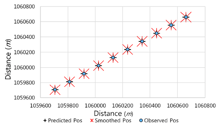
Observed, smoothed and predicted position, No noise
The graph was plotted using the last 10 points as opposed to plotting from the initial state in order to have a clear view of the motion trend of the respective observed, predicted and smoothed tracks. This is especially convenient for the case with noise addition.
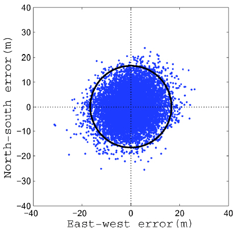
The smoothing and prediction(tracking) errors were calculated by computing the radial distance, 2drms which is twice the root mean square from the observed positions to the smoothed and predicted positions respectively of the circle containing 95% of the total 10000 points. The calculated distances were then sorted in an ascending order that is, from the smallest n = 1 to the largest n = 10000. The radial distance was computed up to the 9500th point. Fig. 2 and Fig. 3 show the 2drms smoothing and prediction errors respectively. In this case they were both equal to zero, that is radius, r = 0(m) , since no noise was added to the system.
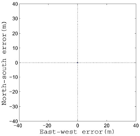
2drms smoothing error, r = 0(m )
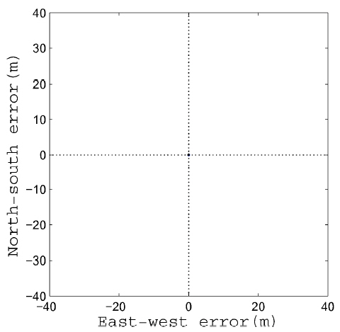
2drms prediction Error, r
4.2 Case 2: Noise present in the system
Gaussian white noise was added to the course and velocity using the matlab function ‘normrnd’. It had a variance of σ2 = 22. Fig. 4 shows the acceleration of the system which remained fairly constant throughout the tracking period whereby the variations were due to noise. This further demonstrates the fact that α – β – γ filter is a constant acceleration filter. Fig. 5 shows the observed, smoothed and predicted positions of the ship while Fig. 6 and 7 show the difference between the observed and smoothed positions and the observed and predicted positions for each time step respectively corresponding to Fig. 5. The difference in the two tracks is due to the noise added to the system. From the figure it is clear that the computed positions, that is, observed, smoothed and predicted positions are not lying on the same track. However, the smoothed positions are closer to the observed positions as compared to the predicted positions which are slightly further away due to error propagation from one point to the next.
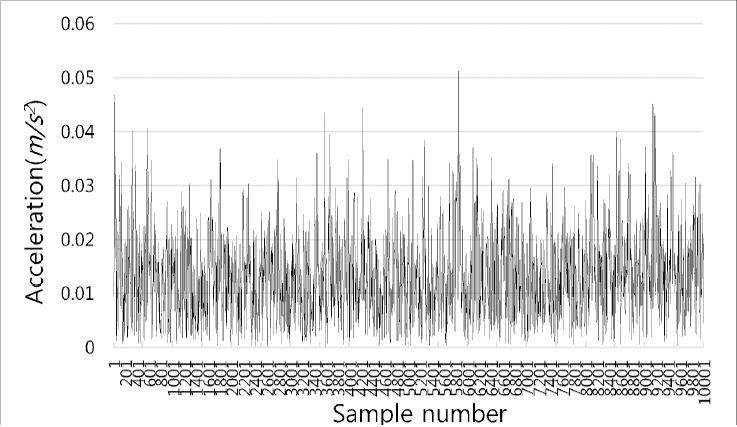
Acceleration, Noisy system, ξ = 0.9
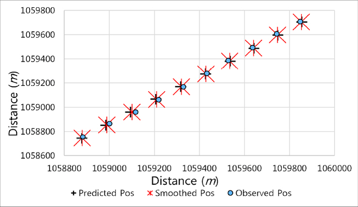
Observed, Smoothed and Predicted Positions, Noise present
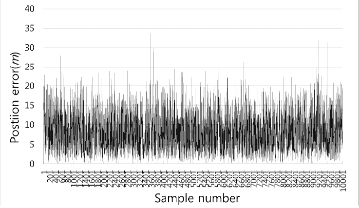
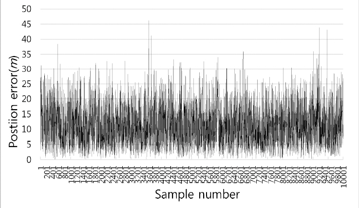
The 2drms error values were computed and plotted as shown in Fig. 8 and Fig. 9. Contrary to the previous case with no noise, an error was present in this case. Fig. 8 and Fig. 9 show the smoothing and prediction 2drms error values respectively. The smoothing error is smaller than the prediction error due to smoothing which reduces the error.
2drms smoothing error, r = 16.6541(m)
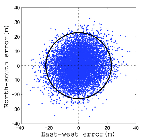
2drms prediction error, r = 22.8451(m)
5 Conclusion
The acceleration in both cases remained fairly constant throughout the tracking period which is true for the α – β – γ filter. The system with no noise maintained its course and had no error as demonstrated in Fig. 2 and Fig. 3 by the 2drms plots whose r = 0(m). The noisy system on the other hand, had a smoothing error of radius, r = 16.6451(m) and a prediction error r = 22.8451(m). The prediction error was larger due to error propagation from one point to the next. The no noise scenario represents an ideal situation hence better results are obtained as compared to the other case with noise. However, in practice, the system must be designed to allow for noise which takes into account the wind, currents and other weather conditions that cause external disturbances. The filter is then applied to compensate for this system noise by reducing it to acceptable levels and subsequently making accurate predictions of the next state. The accuracy of the tracking module was tested by computing the 2drms values of each case. The ideal case was perfect as indicated by the zero error. The noisy scenario, on the other hand, had an error in the tracking and prediction which was, however, managed to an acceptable level.
Future studies will first involve determining the optimum values of α, β and γ parameters required to reduce the noise further while maintaining the stability of the tracking module. Secondly, development of a tracking module where both the target and own ship are on motion will be considered. Finally, a Kalman filter will be designed to examine its accuracy of prediction compared to the α – β – γ filter.